
Sorting is one of the first real problems every programmer runs into. The moment you have a list of numbers, names, or records, you eventually need them arranged in some order. That is where quick sort in data structure comes in.
Quick sort is one of the most popular sorting algorithms taught in computer science courses, and for good reason. It is fast, memory friendly, and shows up again and again in interviews and real software libraries.
At its heart, quick sort picks one element from the array, calls it the pivot, and uses it to split the array into two smaller pieces. Every other element is compared to the pivot and moved to the left or right side depending on whether it is smaller or larger.
In this guide, we will walk through how quick sort works, look at a full example, study the algorithm and its partitioning logic, compare pivot choices, look at time and space complexity, see code in four languages, and finish with common mistakes and frequently asked questions.
What Is Quick Sort in Data Structure?
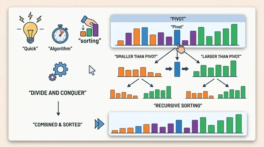
Quick sort is a comparison based sorting algorithm that sorts an array or list by repeatedly dividing it into smaller sub arrays around a chosen pivot element. It was developed by Tony Hoare in 1959 and remains one of the most widely used sorting techniques in modern programming.
The algorithm gets its name simply because it tends to sort data quickly in practice. On average, it beats many other comparison based algorithms when working with arrays, especially large ones that fit in memory.
Quick sort is generally used to sort arrays, but with small modifications it can also work on linked lists and other collections of comparable elements.
The technique it relies on is called divide and conquer, a problem solving approach where a large problem is broken into smaller sub problems, solved independently, and then combined. You can read a broader explanation of this strategy on Wikipedia’s divide and conquer algorithm page.
How Does Quick Sort Work?
The basic idea behind quick sort is simple once you break it into steps. Here is the process in order.
- Select a pivot element from the array.
- Partition the array around that pivot.
- Place all elements smaller than the pivot on its left side.
- Place all elements larger than the pivot on its right side.
- Recursively apply quick sort to the left and right sub arrays.
- Stop the recursion when a sub array has zero or one element, since that is already sorted.
Picture an array as a row of boxes. Every time a pivot is chosen, the row gets split into a smaller row on the left and a smaller row on the right. This splitting keeps happening until every box is sitting in its correct final position.
Quick Sort Example
Let us walk through an example using this array.
[10, 7, 8, 9, 1, 5]
We will use the last element as the pivot for this walkthrough, since that is one of the most common choices in textbooks and code.
- Pivot chosen: 5, which is the last element of the array.
- Every other element is compared with 5.
- Elements smaller than 5, such as 1, are moved toward the left.
- Elements larger than 5, such as 10, 7, 8, and 9, stay on the right side.
- Once every element has been compared, the pivot 5 is placed at its correct sorted position, which is index 1.
- The array is now split into two parts. The left part is [1] and the right part is [7, 8, 9, 10].
- Quick sort is applied again to the right part, choosing a new pivot and repeating the same steps.
- This continues until every sub array has been fully sorted.
The final sorted array becomes:
[1, 5, 7, 8, 9, 10]
Notice how the pivot never moves again once it lands in its correct spot. That single detail is what makes quick sort a genuinely elegant algorithm to trace by hand.
Quick Sort Algorithm
Once you understand the steps, the pseudocode reads almost like plain English.
QUICKSORT(array, low, high)

if low < high
    pivotIndex = PARTITION(array, low, high)

    QUICKSORT(array, low, pivotIndex - 1)
    QUICKSORT(array, pivotIndex + 1, high)
The function takes three inputs, the array itself, and the low and high indices that mark the current sub array being sorted.
If the low index is smaller than the high index, there is more than one element to sort, so partitioning happens first.
The PARTITION function rearranges elements around the pivot and returns the pivot’s final index.
The algorithm then calls itself on the left portion, up to just before the pivot, and separately on the right portion, starting just after the pivot. This recursive call is what makes quick sort a divide and conquer algorithm.
Partitioning in Quick Sort
Partitioning is the real engine of quick sort. Everything else in the algorithm depends on how well this single step is carried out.
Without partitioning, there would be no way to know where the pivot belongs, and the recursive calls on the left and right sides would have nothing meaningful to work with.
How Partitioning Works
- Choose a pivot from the current sub array.
- Compare each remaining element with the pivot value.
- Move every element smaller than the pivot to its left.
- Move every element larger than the pivot to its right.
- Once all comparisons are done, place the pivot in its correct final position between the two groups.
Example of Partitioning
Take a small array: [8, 3, 7, 4, 2]. Using the last element, 2, as the pivot, every element gets compared against it.
Since 8, 3, 7, and 4 are all larger than 2, none of them move to the left. The pivot 2 simply moves to the very front, giving [2, 8, 3, 7, 4].
From here, quick sort would continue on the sub array [8, 3, 7, 4], choosing a new pivot and repeating the same swapping logic.
Pivot Selection in Quick Sort
The pivot is arguably the single most important choice in quick sort. A good pivot creates two roughly equal halves, while a poor one can create a badly unbalanced split.
There are several common strategies for picking a pivot.
- First element: simple to implement, but risky on already sorted data.
- Last element: the most common textbook choice, used in the Lomuto partition scheme.
- Middle element: often a safer middle ground for partially sorted arrays.
- Random element: helps avoid predictable worst case patterns, especially in competitive programming.
- Median of three: compares the first, middle, and last elements, then picks the median of the three as the pivot.
Pivot selection directly affects performance. A pivot close to the median of the data produces balanced partitions and keeps quick sort close to its best case speed. A consistently poor pivot, such as always picking the smallest or largest element in a sorted array, pushes the algorithm toward its slower worst case.
Types of Partitioning in Quick Sort
Two partitioning schemes show up most often in textbooks and interviews. Knowing both gives you a deeper, more complete picture of quick sort.
Lomuto Partition Scheme
The Lomuto scheme is the simpler of the two and is usually the first one students learn.
- Basic idea: the pivot is usually the last element of the sub array.
- How it works: a pointer tracks the boundary of elements smaller than the pivot, and the array is scanned left to right, swapping smaller elements into place as they are found.
- When it is commonly used: introductory courses and simple implementations, since the logic is easy to follow and code.
Hoare Partition Scheme
The Hoare scheme was actually the original partitioning method proposed by Tony Hoare himself.
- Basic idea: two pointers start at opposite ends of the sub array and move toward each other.
- How it differs from Lomuto: instead of placing the pivot in its exact final position immediately, it simply ensures elements on the left are not greater than the pivot and elements on the right are not smaller.
- Why it can perform fewer swaps: because both pointers move inward and stop only when a swap is genuinely needed, Hoare’s method typically does about three times fewer swaps than Lomuto on average.
Quick Sort Time and Space Complexity
Understanding complexity helps explain why quick sort is fast in practice but not always guaranteed to be fast.
| Case | Time Complexity |
|---|---|
| Best Case | O(n log n) |
| Average Case | O(n log n) |
| Worst Case | O(n²) |
Balanced partitions produce O(n log n) performance because each recursive split roughly halves the problem size, similar to how merge sort behaves.
Poor pivot selection, on the other hand, can result in O(n²) performance. This happens when the pivot repeatedly turns out to be the smallest or largest element, producing one sub array with almost all the elements and another with almost none. Wikipedia’s quicksort article covers this worst case scenario in more mathematical detail, including sorted or reverse sorted arrays as classic trigger cases.
Because quick sort is recursive, it also uses stack space for each recursive call. In the best and average cases, this stack depth stays around O(log n). In the worst case, where partitions are highly unbalanced, the recursion depth can grow to O(n).
This is the key difference between average and worst case performance. Average case behavior assumes reasonably balanced splits, while worst case behavior assumes the most unfavorable pivot choices happen again and again.
Quick Sort Implementation
Seeing the algorithm in actual code often makes it click faster than pseudocode alone. Below are clean implementations in four widely used languages, each using the Lomuto partition scheme with the last element as the pivot.
Quick Sort in C
#include <stdio.h>

void swap(int* a, int* b) {
    int t = *a; *a = *b; *b = t;
}

int partition(int arr[], int low, int high) {
    int pivot = arr[high];
    int i = low - 1;
    for (int j = low; j < high; j++) {
        if (arr[j] < pivot) {
            i++;
            swap(&arr[i], &arr[j]);
        }
    }
    swap(&arr[i + 1], &arr[high]);
    return i + 1;
}

void quickSort(int arr[], int low, int high) {
    if (low < high) {
        int pi = partition(arr, low, high);
        quickSort(arr, low, pi - 1);
        quickSort(arr, pi + 1, high);
    }
}
The partition function tracks a boundary index i, moving it forward every time a smaller element is found and swapping it into place. Once the loop ends, the pivot itself is swapped into its correct spot. The recursive calls then sort everything to its left and right. Running this on [10, 7, 8, 9, 1, 5] produces the output 1 5 7 8 9 10.
Quick Sort in C++
#include <bits/stdc++.h>
using namespace std;

int partition(vector<int>& arr, int low, int high) {
    int pivot = arr[high];
    int i = low - 1;
    for (int j = low; j < high; j++) {
        if (arr[j] < pivot) {
            i++;
            swap(arr[i], arr[j]);
        }
    }
    swap(arr[i + 1], arr[high]);
    return i + 1;
}

void quickSort(vector<int>& arr, int low, int high) {
    if (low < high) {
        int pi = partition(arr, low, high);
        quickSort(arr, low, pi - 1);
        quickSort(arr, pi + 1, high);
    }
}
This version uses the standard library’s swap function and a vector instead of a raw array, which is the more common style in modern C++. The partition logic is identical to the C version. For the same input array, the expected output is 1 5 7 8 9 10.
Quick Sort in Java
public class QuickSort {
    static void swap(int[] arr, int a, int b) {
        int t = arr[a]; arr[a] = arr[b]; arr[b] = t;
    }

    static int partition(int[] arr, int low, int high) {
        int pivot = arr[high];
        int i = low - 1;
        for (int j = low; j < high; j++) {
            if (arr[j] < pivot) {
                i++;
                swap(arr, i, j);
            }
        }
        swap(arr, i + 1, high);
        return i + 1;
    }

    static void quickSort(int[] arr, int low, int high) {
        if (low < high) {
            int pi = partition(arr, low, high);
            quickSort(arr, low, pi - 1);
            quickSort(arr, pi + 1, high);
        }
    }
}
Java’s version follows the exact same partition and recursive call structure, just wrapped inside a class since Java requires methods to live inside one. Calling quickSort on [10, 7, 8, 9, 1, 5] with low as 0 and high as arr.length minus 1 produces the sorted output 1 5 7 8 9 10.
Quick Sort in Python
def partition(arr, low, high):
    pivot = arr[high]
    i = low - 1
    for j in range(low, high):
        if arr[j] < pivot:
            i += 1
            arr[i], arr[j] = arr[j], arr[i]
    arr[i + 1], arr[high] = arr[high], arr[i + 1]
    return i + 1

def quick_sort(arr, low, high):
    if low < high:
        pi = partition(arr, low, high)
        quick_sort(arr, low, pi - 1)
        quick_sort(arr, pi + 1, high)
Python’s tuple based swapping, arr[i], arr[j] = arr[j], arr[i], makes the partition function noticeably shorter than in C, C++, or Java. The recursive calls and overall logic remain exactly the same. Calling quick_sort on [10, 7, 8, 9, 1, 5] with low as 0 and high as len(arr) minus 1 gives the expected sorted output of 1 5 7 8 9 10.
Advantages of Quick Sort
- Average case performance of O(n log n), which is fast for most real world datasets.
- Efficient for large datasets that fit comfortably in memory.
- Usually requires less additional memory than merge sort when implemented in place.
- Works especially well with arrays, thanks to good cache locality.
- Follows the divide and conquer approach, which makes it easy to reason about and parallelize.
Disadvantages of Quick Sort
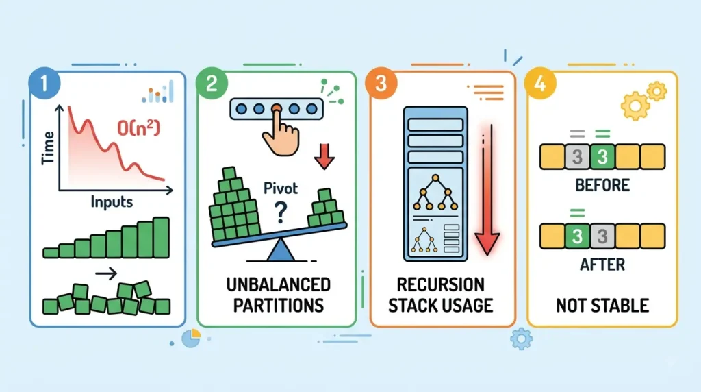
- Worst case time complexity of O(n²), which can appear on already sorted or specially crafted inputs.
- Performance depends heavily on pivot selection.
- Recursive implementation can increase stack usage, especially with unbalanced partitions.
- The basic version of quick sort is not stable, meaning equal elements might not keep their original relative order.
- Poor pivot choices can make the algorithm noticeably inefficient on certain patterns of data.
Quick Sort vs Other Sorting Algorithms
A side by side comparison makes the trade offs easier to see at a glance.
| Feature | Quick Sort | Merge Sort | Bubble Sort | Insertion Sort |
|---|---|---|---|---|
| Best Case | O(n log n) | O(n log n) | O(n) | O(n) |
| Average Case | O(n log n) | O(n log n) | O(n²) | O(n²) |
| Worst Case | O(n²) | O(n log n) | O(n²) | O(n²) |
| Approach | Divide and conquer | Divide and conquer | Comparison | Comparison |
| Stable | No | Yes | Yes | Yes |
| Extra Space | Low for in place version | Higher | Low | Low |
Applications of Quick Sort
- Sorting arrays in general purpose programs.
- Powering many built in sorting functions across programming languages.
- Acting as a preprocessing step before searching algorithms that need sorted data.
- Handling large datasets where average case performance matters more than worst case guarantees.
- Solving problems in algorithm courses and coding assessments.
- Appearing frequently in competitive programming and coding interviews.
Quick Sort vs Merge Sort: Which Is Better?
This is one of the most common questions students ask, and the honest answer is that neither algorithm is always better. It really depends on what the situation calls for.
- Quick sort can be faster in practice for many in memory arrays, thanks to good cache behavior and lower constant factors.
- Merge sort provides predictable O(n log n) performance in every case, including the worst case.
- Merge sort is the better pick when stability is required, such as when sorting records by one field while preserving the original order of ties.
- Quick sort is often preferable when minimizing additional memory usage matters, since it can be implemented in place.
In short, reach for quick sort when average speed and low memory use matter most, and reach for merge sort when consistency and stability matter most.
Common Mistakes in Quick Sort
These are the errors that trip up most students and even experienced developers when implementing quick sort for the first time.
- Choosing a poor pivot repeatedly, such as always picking the first or last element on nearly sorted data.
- Setting incorrect partition boundaries, which can leave elements out of the sort entirely.
- Forgetting the base condition, causing infinite or excessive recursion.
- Using incorrect recursive ranges, such as passing the wrong low or high index.
- Ending up with infinite recursion because the pivot index was calculated incorrectly.
- Mishandling duplicate elements, which can cause unnecessary or incorrect swaps.
- Confusing pivot selection with partitioning, treating them as the same step when they are actually two separate operations.
Frequently Asked Questions About Quick Sort
What is quick sort in data structure?
Quick sort is a comparison based sorting algorithm that divides an array around a pivot element and recursively sorts the resulting sub arrays until the entire structure is sorted.
Why is quick sort called a divide and conquer algorithm?
Because it breaks a large sorting problem into smaller sub problems, solves each one recursively, and relies on the fact that sorting the smaller pieces automatically sorts the whole array once the pivot is in place.
What is a pivot in quick sort?
A pivot is the element chosen from the array that all other elements are compared against during partitioning. Its final position separates the smaller elements from the larger ones.
What is the average time complexity of quick sort?
The average time complexity of quick sort is O(n log n), assuming reasonably balanced partitions across the recursive calls.
What is the worst case time complexity of quick sort?
The worst case time complexity is O(n²), which typically occurs when the pivot is repeatedly the smallest or largest remaining element.
Is quick sort stable?
The standard version of quick sort is not stable, since elements with equal values are not guaranteed to keep their original relative order after sorting.
Is quick sort faster than merge sort?
In practice, quick sort is often faster on average for in memory arrays because of lower memory overhead and better cache performance, though merge sort offers more predictable worst case behavior.
What happens when the pivot is the smallest or largest element?
The array gets split very unevenly, with one sub array holding almost all the elements and the other holding almost none. Repeating this pattern leads to the O(n²) worst case.
Which pivot is best for quick sort?
There is no single best pivot for every situation, but the median of three approach or a randomly chosen pivot tends to give consistently balanced partitions across a wide range of inputs.
Where is quick sort used?
Quick sort is used in general purpose sorting libraries, academic algorithm courses, competitive programming, and any scenario where fast average case sorting of arrays is needed.
Conclusion
Quick sort in data structure remains one of the most practical sorting algorithms you can learn, precisely because it blends simple logic with genuinely strong real world performance.
Everything in the algorithm revolves around two ideas: choosing a sensible pivot and partitioning the array correctly around it. Get those two steps right, and the recursive calls take care of the rest.
On average, quick sort delivers O(n log n) performance, though a poorly chosen pivot can push it toward the slower O(n²) worst case. This is exactly why pivot selection strategies, such as random or median of three pivots, matter so much in production quality implementations.
Whether you are studying for exams, preparing for coding interviews, or simply trying to understand how programming languages sort data behind the scenes, quick sort is an algorithm worth truly understanding rather than just memorizing.