
To freeze a row in Excel, open the View tab, select Freeze Panes, and choose Freeze Top Row. Row 1 now stays visible while you scroll. That is the whole trick for the most common case.
Freeze Panes lock rows or columns in place so your headers don’t disappear when you scroll through a long worksheet. If you have ever lost track of which column holds “Revenue” and which holds “Region” at row 400, this feature fixes that. This guide covers every version of the task: one row, several rows, rows and columns together, different platforms, unfreezing, and what to do when it misbehaves.
How to Freeze the Top Row in Excel
Freezing the top row is the fastest option because Excel has a dedicated command for it. You don’t need to select any cell first.
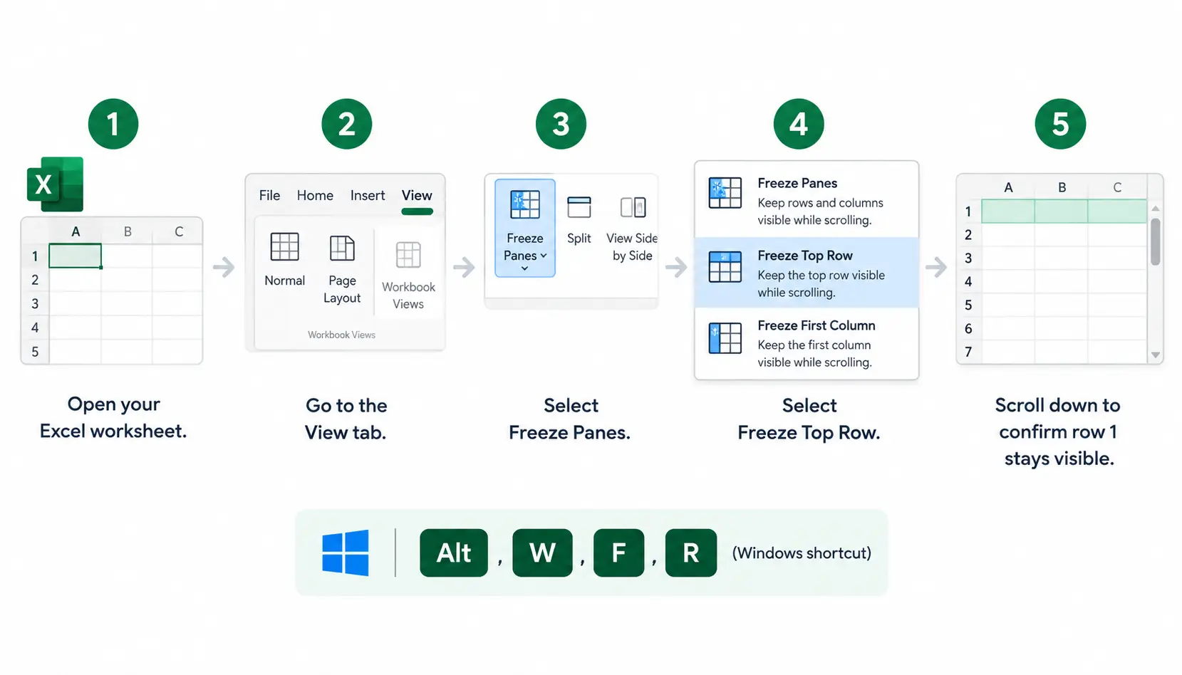
Steps to freeze the first row
- Open your Excel worksheet.
- Go to the View tab.
- Select Freeze Panes.
- Select Freeze Top Row.
- Scroll down to confirm that row 1 stays visible.
On Windows, you can also press Alt, W, F, R in sequence as a keyboard shortcut for the same command.
How to tell if the row is frozen
Look at the line under row 1. A frozen row shows a slightly darker, thicker boundary than the normal gridlines. It is easy to miss on some screens, so don’t rely on it alone.
The real test is scrolling. Move down the sheet. The frozen row stays at the top while every other row slides underneath it. If row 1 scrolls away, the freeze did not apply.
How to Freeze Multiple Rows in Excel
The Freeze Top Row button only handles row 1. To freeze more than one row, you use the general Freeze Panes command and tell Excel where the freeze line goes by selecting a cell first.
Excel freezes everything above and to the left of the cell you select. Remember that one rule and the rest is easy.
How to freeze the first two rows
Select cell A3, then go to View → Freeze Panes → Freeze Panes. Rows 1 and 2 are now locked.
This is handy when row 1 holds a report title and row 2 holds your column headers.
How to freeze the first three rows
Select cell A4, then go to View → Freeze Panes → Freeze Panes. Rows 1 to 3 are now locked.
How to freeze any number of top rows
Use this rule: select the row immediately below the last row you want to freeze. You can click the row number or just click a cell in column A of that row.
Want to freeze 5 rows? Select A6. Want 8 rows? Select A9. The pattern never changes.
How to Freeze a Row and Column at the Same Time
Wide spreadsheets need both. You want headers on top and an identifier, such as a name or product code, on the left. Excel lets you lock both in one step.
Freeze the top row and first column
Select cell B2, then go to View → Freeze Panes → Freeze Panes. Row 1 and column A are now locked.
B2 works because it sits just below row 1 and just right of column A.
Freeze multiple rows and columns
Select cell C4 to freeze rows 1 to 3 and columns A to B. The same above-and-left rule applies, just with bigger numbers.
Quick reference table
| Desired frozen area | Cell to select |
| Row 1 | A2 |
| Rows 1–2 | A3 |
| Rows 1–3 | A4 |
| Row 1 + Column A | B2 |
| Rows 1–3 + Columns A–B | C4 |
How to Freeze the First Column in Excel
Sometimes you only need the left side to stay put, for example when you scroll across months of data and want to keep sight of each customer name.
Freeze only column A
Go to View → Freeze Panes → Freeze First Column. No cell selection is needed.
Freeze multiple columns
The same selection principle applies. Select the column immediately to the right of the last column you want to freeze.
For example, select C1, then go to View → Freeze Panes → Freeze Panes to lock columns A and B.
How to Freeze Rows in Excel for Different Platforms
The core steps are almost identical everywhere. The menus look slightly different, so here is what to expect.
Excel for Windows
Open the View tab on the ribbon. In the Window group, click Freeze Panes. Choose Freeze Top Row, Freeze First Column, or Freeze Panes for a custom freeze point.
Excel for Mac
Mac users also use the View tab and the Freeze Panes button. The dropdown offers the same three choices: top row, first column, and a custom frozen area based on your selected cell. Microsoft documents this on its Freeze panes support page.
Excel for the web
Excel for the web also supports Freeze Panes from the ribbon under the View tab. The wording can differ a little from the desktop app, and a few advanced view features are limited in the browser. If you need something the web version doesn’t offer, open the file in the desktop app.
Microsoft 365 vs older Excel versions
The Freeze Panes workflow is very similar across Microsoft 365 and older supported versions of Excel. Menu names and ribbon layouts can shift between releases, but the idea is the same: pick a cell, then freeze above and to the left of it.
How to Unfreeze Rows or Columns in Excel
Removing a freeze takes seconds.
Steps to unfreeze panes
- Go to the View tab.
- Select Freeze Panes.
- Select Unfreeze Panes.
This removes all frozen rows and columns on the active sheet. Microsoft lists this as the standard method.
How to change which rows are frozen
Excel does not let you nudge a freeze line. Instead, do this:
- Unfreeze the panes.
- Select the correct cell.
- Apply Freeze Panes again.
Why Freeze Panes Isn’t Working in Excel
When Freeze Panes acts strangely, the cause is usually one of the five issues below.
You’re selecting the wrong cell
This is the most common mistake. Excel freezes what is above and to the left of your selection. If you select A1, there is nothing above or to the left, so the result looks wrong. Pick the cell just below the rows and just right of the columns you want to lock.
Another pane is already frozen
If an earlier freeze is still active, the new one can behave in confusing ways. Unfreeze first, then set the new freeze point.
Freeze Panes is grayed out
A grayed-out button usually points to the current view or mode. Common causes include:
- The worksheet is in the Page Layout view. Switch to Normal view from the View tab.
- You are in the middle of editing a cell. Press Enter or Esc first.
- You are using a limited platform or view, such as some web or protected-file situations.
Excel is freezing more rows than expected
Excel freezes from the top of what you can currently see. If you scrolled down before freezing, rows above your screen can end up hidden. Scroll back to the very top (press Ctrl + Home on Windows) before you select your cell. Then, for example, select A3 to freeze only rows 1 and 2.
You’re using Freeze Top Row when you need custom rows
Freeze Top Row locks row 1 only, no matter what is selected. If your headers are in row 4, you need the general Freeze Panes command with A5 selected instead.
Freeze Panes vs Split Panes vs Protect Sheet
These three features sound related, but they solve different problems.
Freeze Panes
Keep chosen rows or columns visible while you scroll through the rest of the sheet.
Split Panes
Splits the window into separate scrollable areas, so you can view two parts of the same sheet at once. Microsoft documents Split as its own feature, also found on the View tab.
Protect Sheet
Controls whether people can edit certain cells. It has nothing to do with scrolling.
Comparison table
| Feature | What it does | Best for |
| Freeze Panes | Locks rows/columns in view while scrolling | Keeping headers visible |
| Split Panes | Creates independent scrolling areas | Comparing distant parts of one sheet |
| Protect Sheet | Restricts editing | Preventing accidental changes |
Practical Examples of When to Freeze Rows in Excel
1. Large sales reports
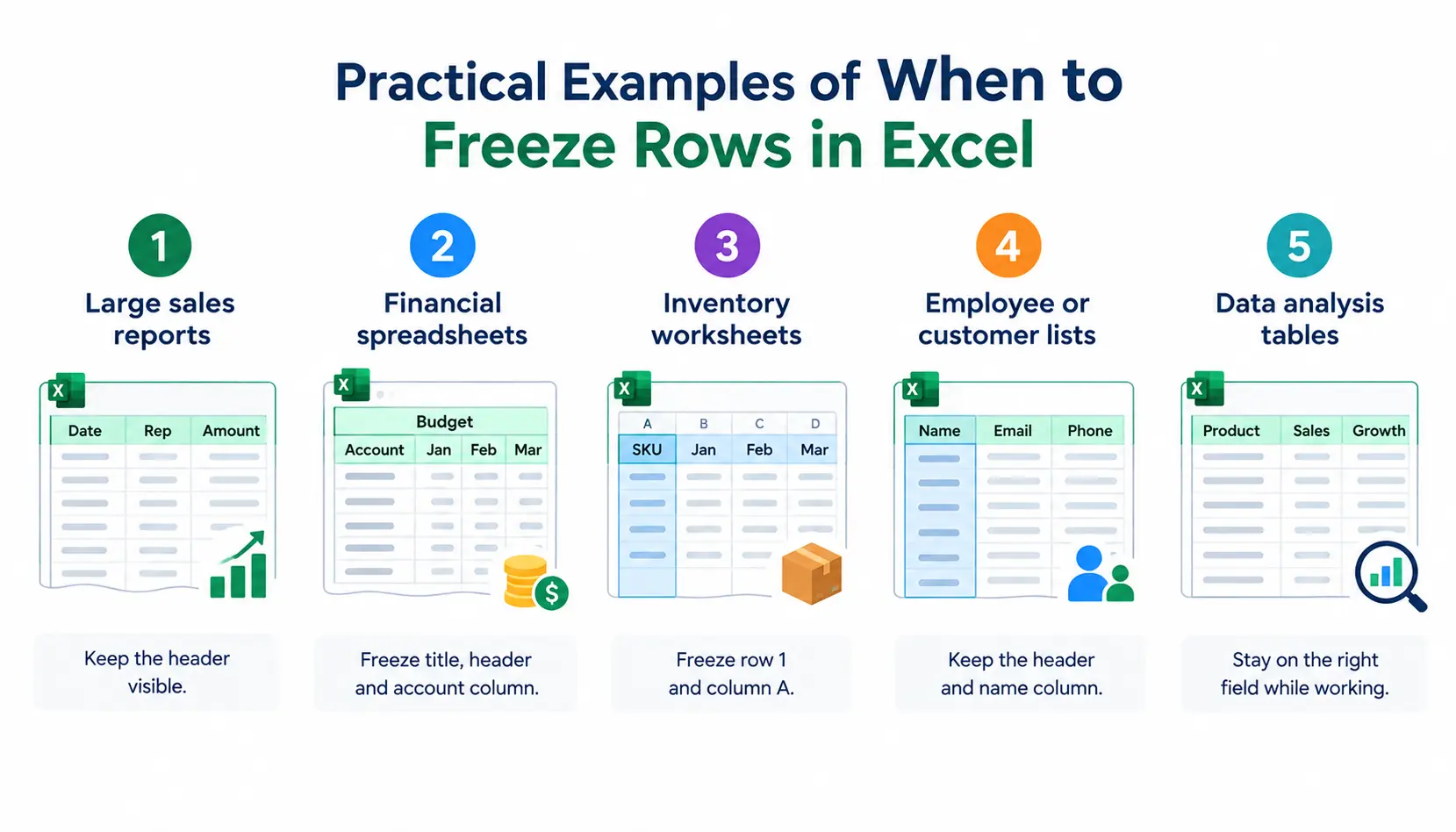
A monthly sales export can run to thousands of lines. Freeze the header row so “Date,” “Rep,” and “Amount” stay visible all the way down.
2. Financial spreadsheets
Budgets often have a title row and a header row. Freeze both, and freeze the account name column so line items stay readable as you scroll right through the months.
3. Inventory worksheets
With SKUs on the left and stock levels across many columns, freezing row 1 and column A keeps every number tied to its product.
4. Employee or customer lists
Freeze the header row and the name column. You can scroll through contact details without guessing whose row you are on.
5. Data analysis tables
When you filter, sort, or build formulas against a large table, frozen headers help you avoid mistakes. You always see which field you are working with.
Tips for Using Freeze Panes Effectively
Keep header rows concise
Frozen rows take up screen space. Short, single-line headers leave more room for your data, especially on laptops.
Freeze only what you need
Freezing too many rows can leave almost no scrolling area. If your frozen section fills half the screen, trim it.
Combine frozen rows with a frozen identifier column
For wide tables, lock the top row and the key column together. Select B2 and freeze, and you get both.
Check the freeze boundary before working with large datasets
Scroll a little right after applying the freeze. A quick test saves you from discovering the wrong setup 2,000 rows later.
Unfreeze and reset when changing worksheet layouts
If you insert title rows or restructure the sheet, unfreeze and set the freeze point again. An old freeze line can end up in the wrong place.
Frequently Asked Questions About Freezing Rows in Excel
1. How do I freeze a row in Excel?
Go to View → Freeze Panes → Freeze Top Row to lock row 1. For any other row, select the cell below it in column A and choose Freeze Panes.
2. How do I freeze the top two rows?
Select cell A3, then go to View → Freeze Panes → Freeze Panes.
3. How do I freeze multiple rows?
Select the row immediately below the last row you want to freeze, then choose View → Freeze Panes → Freeze Panes.
4. Can I freeze a row and column together?
Yes. Select the cell just below the row and just right of the column you want to lock. For row 1 and column A, that is B2.
5. How do I unfreeze a row?
Go to View → Freeze Panes → Unfreeze Panes.
6. Does freezing a row prevent editing?
No. Freezing only changes how the sheet scrolls. You can still edit frozen cells. To block edits, use Protect Sheet.
7. Can I freeze rows in Excel for the web?
Yes. Excel for the web supports Freeze Panes from the View tab on the ribbon.
8. Why is Excel freezing the wrong rows?
Usually you selected the wrong cell, or you scrolled down before freezing. Unfreeze, scroll to the top, select the cell just below the rows you want, and freeze again.
9. What is the difference between Freeze Panes and Split Panes?
Freeze Panes keeps certain rows or columns fixed while the rest scrolls. Split Panes divides the window into separate areas that each scroll on their own.
Conclusion
Learning how to freeze a row in Excel takes less than a minute, and it saves time every day you work with long data. For row 1, use View → Freeze Panes → Freeze Top Row. For anything else, select the cell below and to the right of what you want locked, then choose Freeze Panes.
If something goes wrong, unfreeze and start again. The mistake is almost always the selected cell.