
The Excel shortcut for SUM on Windows is Alt + =. Select the cell where you want the total, press the keys, and Excel inserts a SUM formula for you.
That key combination triggers AutoSum. It looks at the cells around your selection and guesses which numbers you want to add. Most of the time it guesses right. When it doesn’t, you can fix the range before you confirm, and this guide shows you how.
On Mac, the equivalent is Command + Shift + T.
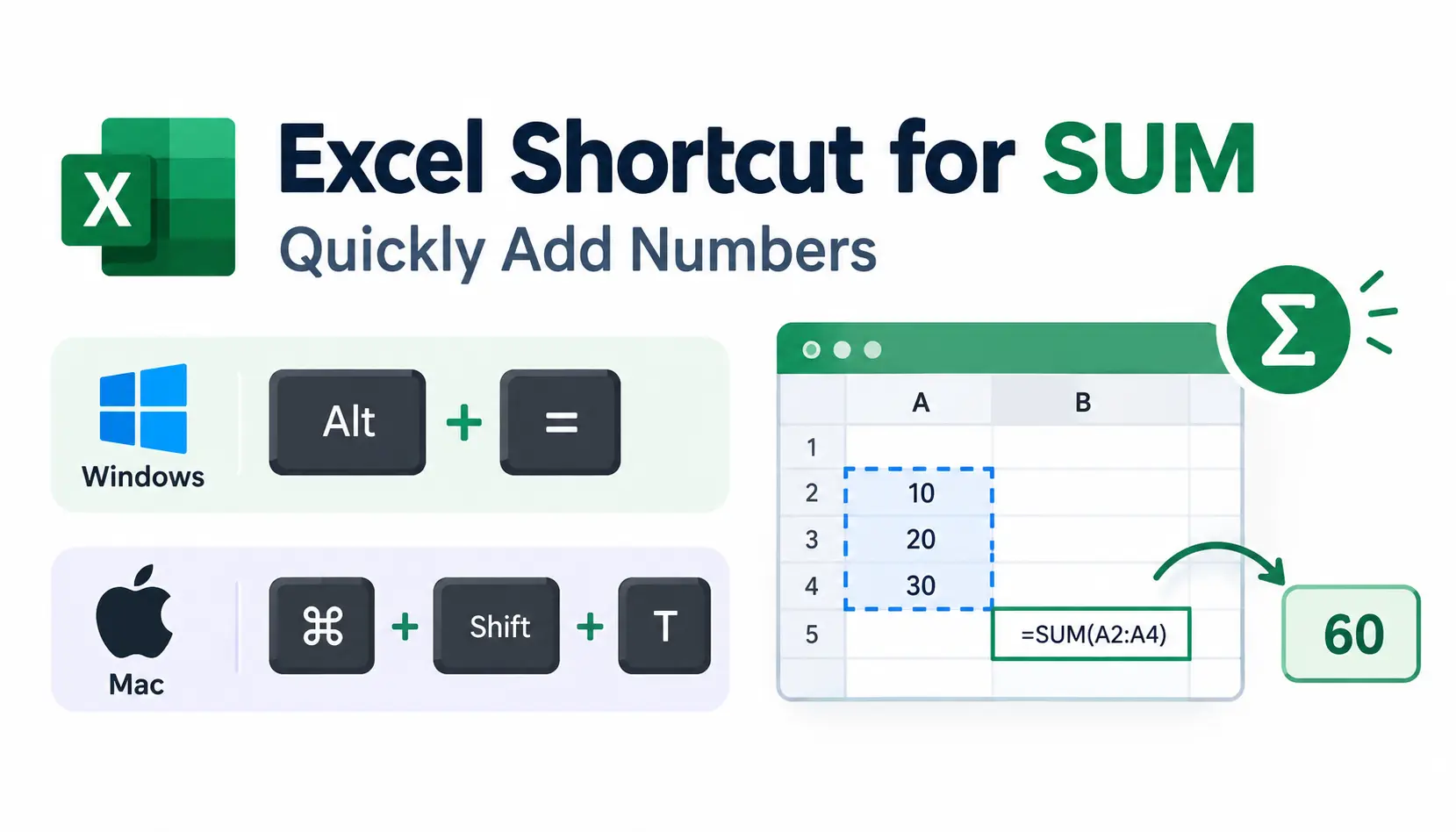
What Is the Excel Shortcut for SUM?
There is one main shortcut, and it works the same way every time you use it. Learn it once and you will save a few seconds on every total you build.
Windows SUM shortcut
Press Alt + = (hold Alt, then press the equals key). On most keyboards the equals key sits next to Backspace. Some laptops need the Fn key as well.
You do not need to type a single character of the formula. Excel writes it for you.
What the shortcut actually does
Alt + = runs the AutoSum command, the same one behind the Σ button on the Home tab. Excel scans up the column first, then to the left along the row. It picks the nearest block of numbers and wraps it in a SUM function.
The formula appears in the cell with the range highlighted by a moving border. Nothing is final until you press Enter. That pause gives you a chance to check the work.
AutoSum does not invent anything new. It simply types a standard SUM formula for you, which means you can edit it like any other formula afterward.
Example
Say you track monthly sales in this small table:
| A | B | |
| 1 | Month | Sales |
| 2 | January | 120 |
| 3 | February | 180 |
| 4 | March | 150 |
| 5 | Total |
Click cell B5 and press Alt + =. Excel fills in =SUM(B2:B4) and highlights B2:B4. Press Enter, and B5 shows 450.
Notice that Excel skipped the header in B1. It stops at text, so it knew where your numbers began.
How to Use the AutoSum Shortcut in Excel
The process is the same for any list of numbers. Four steps, and the whole thing takes a couple of seconds.
Step 1: Select the total cell
Click the empty cell directly below a column of numbers, or directly to the right of a row of numbers. AutoSum looks in those two directions first.
Step 2: Press Alt + =
Excel types the formula and highlights the range it chose. The cell is now in edit mode.
Step 3: Check the selected range
Look at the highlighted border. Does it cover every number you want, and nothing else? If not, drag the border or type the correct range.
Step 4: Press Enter
Enter confirms the formula and shows the result. If you want to stay in the same cell, press Ctrl + Enter instead.
Warning: Always check the highlighted range before you confirm the formula. A total that quietly leaves out a row is worse than no total at all, because nobody questions it.
How to Sum a Column With the Excel Shortcut
Columns are where this shortcut earns its keep. Here are the three situations you will meet most often.
Sum numbers directly above a cell
Click the cell under the last number and press Alt + =. In the sales example above, that is B5. Excel adds everything above it until it hits a blank cell or a text label.
Sum an entire column
If you want the total of a whole column, including numbers you add later, type the formula yourself:
=SUM(B:B)
Put it in a different column or above the data. If you place it inside column B, you create a circular reference, and Excel will warn you.
Sum multiple columns
Suppose you have sales in column B, costs in column C, and profit in column D, with data in rows 2 to 4. Select B5:D5 (the three empty cells below the data) and press Alt + =. Excel fills a SUM formula into each cell at once.
You can also select the data and the empty row together, for example B2:D5, then press Alt + =. This is the fastest way to total a whole table.
How to Sum a Row With the Excel Shortcut
Rows work the same way, only Excel looks to the left instead of upward.
Sum numbers to the left of a cell
Here is a quarterly layout:
| A | B | C | D | E | |
| 1 | Product | Jan | Feb | Mar | Total |
| 2 | Pens | 40 | 55 | 60 |
Click E2 and press Alt + =. Excel writes =SUM(B2:D2) and highlights the three months. Press Enter to get 155.
Sum multiple rows
Select the empty total cells for several rows at once, such as E2:E10, and press Alt + =. Every row gets its own SUM formula. You can also select the whole block, including the total column, and press the shortcut once.
If you want row totals and column totals together, select the full block plus one extra row and one extra column. Alt + = fills both.
How to Fix Excel When AutoSum Selects the Wrong Range
AutoSum is a guess, and guesses sometimes miss. The good news is that the fix is simple: change the range while the formula is still in edit mode.
To adjust the range, drag the corner handles of the highlighted border. Or click inside the formula and type the new range by hand. Press Enter once it looks right.
Excel includes too many cells
This usually happens when a number sits above your data, such as a year in a header. Excel treats it as part of the list. Shrink the range so it starts at the first real data cell.
Excel misses cells
If the range stops short, there is usually a gap in the data. Extend the range by dragging the border to the last cell you need.
Blank cells interrupt the range
AutoSum stops at the first blank cell it meets. If your column has gaps, you will get a partial total. Either fill the gaps, or type the full range yourself, like =SUM(B2:B20). SUM ignores blank cells inside a range, so it handles gaps fine once you set the range.
Text or labels appear near the numbers
Subtotal labels, notes, or section headings can confuse the guess. If Excel picks the wrong block, correct it by hand. A habit worth building: glance at the highlighted border every time, even when you are in a hurry.
How to Enter the SUM Formula Manually
AutoSum is fast, but typing the formula gives you full control. The basic version is:
=SUM(B2:B10)
This adds every number from B2 to B10.
Sum individual cells
Use commas to pick specific cells that are not next to each other:
=SUM(B2,B5,B9)
Sum multiple ranges
You can combine separate blocks in one formula:
=SUM(B2:B10,D2:D10)
Manual formulas are better in a few cases. Use them when your data has gaps, when the cells you need are scattered, or when you want to total a range that does not sit next to the formula cell. They also help when you want the formula to cover rows you have not filled in yet.
Microsoft documents the full syntax on its SUM function support page.
AutoSum vs. SUM: What’s the Difference?
People often treat these as two separate tools. They are not. AutoSum is a quick way to create a SUM formula. Once you press Enter, the cell holds a regular SUM function either way.
| Feature | AutoSum | SUM |
| Main purpose | Quickly create a SUM formula | Manually create a SUM formula |
| Keyboard shortcut | Alt + = | Type =SUM() |
| Automatic range detection | Yes | No |
| Best for | Fast totals | Precise formulas |
The real difference is who picks the range. With AutoSum, Excel guesses. With SUM typed by hand, you decide.
Other Ways to Quickly Sum Numbers in Excel
The shortcut is not the only quick option. Depending on the job, one of these may suit you better.
Use the AutoSum button
Go to Home, then click AutoSum (the Σ symbol) in the Editing group. It does exactly what Alt + = does. The Formulas tab has the same button.
Use the status bar
Select a group of numeric cells and look at the bottom-right of the Excel window. The status bar shows the sum, the average, and the count by default. This is perfect for a quick check because it does not put anything in your sheet.
If you do not see these values, right-click the status bar and turn them on.
Use the Formula Bar
Click any total and look at the formula bar above the grid. It shows the exact range being added. This is the easiest way to audit a formula, or to edit it without double-clicking the cell. If you’re working with a large worksheet, you can also freeze a row in Excel to keep column headers visible while you scroll through your data.
How to Sum Filtered Data in Excel
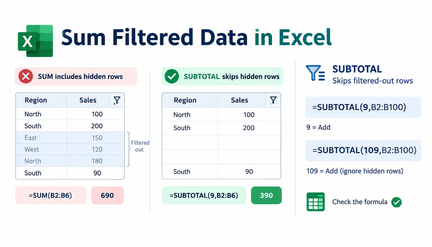
Ordinary SUM adds every cell in the range, including rows that a filter has hidden. That surprises many people. You filter a list down to one region, yet the total still shows all regions.
When to use SUBTOTAL instead
The SUBTOTAL function can skip filtered-out rows:
=SUBTOTAL(9,B2:B100)
The number 9 tells Excel to add. Use 109 instead if you also want to ignore rows you hid by hand. Excel’s own AutoSum usually switches to SUBTOTAL when it detects a filtered list, but it is wise to check the formula.
See Microsoft’s SUBTOTAL function page for the full list of function numbers.
Using AutoSum With Excel Tables
Excel Tables add structure to your data, and they make totals easier. If you work with lists that grow, Tables are worth learning.
Convert the range to a Table
Click anywhere in your data and press Ctrl + T. Confirm that the range is correct and tick the box if your data has headers.
Add a Total Row
With a cell in the table selected, go to Table Design and tick Total Row. You can also press Ctrl + Shift + T. Excel adds a row at the bottom with a dropdown in each cell, so you can choose Sum, Average, Count, and more.
The Total Row uses SUBTOTAL behind the scenes, so it responds correctly to filters.
Use structured references
Inside a Table, formulas use column names instead of cell addresses:
=SUM(Table1[Sales])
This formula keeps working when you add rows, because the Table expands automatically. It is also easier to read than B2:B100. Table1 is the default name, so rename yours for clarity.
Common Problems With the Excel SUM Shortcut
Most issues fall into a handful of causes. Here is how to spot and fix each one.
Alt + = doesn’t work
First, make sure you are not already typing in a cell. Press Esc, then try again. Some laptops need Fn held down to reach the equals key. Check your keyboard language too, since a different layout can move the equals sign. On Mac, use Command + Shift + T instead.
Excel selects the wrong cells
This is the range-guess problem covered earlier. Edit the highlighted range before pressing Enter.
The result is zero
The usual cause is numbers stored as text. Another cause is calculation set to manual: check Formulas, then Calculation Options, and choose Automatic.
Numbers are stored as text
Text numbers often sit on the left side of a cell and may show a small green triangle. Click the warning icon and choose Convert to Number. For a whole column, select it, then use Data, then Text to Columns, and click Finish.
The formula displays instead of the result
The cell is probably formatted as Text. Change the format to General, then click the cell and press Enter again. Also check whether Show Formulas is on. Press Ctrl + ` to toggle it.
Hidden or filtered rows affect the result
SUM counts hidden rows. If you want only visible rows, use SUBTOTAL as shown above.
Excel SUM Shortcuts and Related Functions
Use this table as a quick reference when you are not sure which tool to pick.
| Need | Best option |
| Quickly total nearby numbers | AutoSum |
| Manually total a range | SUM |
| Sum with one condition | SUMIF |
| Sum with multiple conditions | SUMIFS |
| Sum visible/filtered data | SUBTOTAL |
If you are new to the wider spreadsheet world, Wikipedia has a helpful overview of Microsoft Excel. For real-world questions and troubleshooting from other users, the excel community on Reddit is an active place to ask. If you’re building your spreadsheet skills from the ground up, this guide to free online computer courses with certificates can help you find broader computer and data-learning resources.
Excel SUM Shortcut FAQs
1. What is the shortcut for SUM in Excel?
On Windows, press Alt + =. On Mac, press Command + Shift + T. Both insert a SUM formula using AutoSum.
2. What does Alt + = do in Excel?
It runs AutoSum. Excel detects the nearby numbers, writes a SUM formula, and highlights the range so you can confirm it.
3. How do I quickly sum a column?
Click the empty cell below the numbers and press Alt + =. Check the highlighted range, then press Enter.
4. How do I quickly sum a row?
Click the empty cell to the right of the numbers and press Alt + =. Excel sums the cells to the left.
5. Why does AutoSum select the wrong range?
Excel stops at blank cells and may include numbers in headers. Edit the range while the formula is still active, then press Enter.
6. Can I use AutoSum on multiple columns?
Yes. Select the empty cells under all the columns you want to total, then press Alt + =. Excel fills a formula into each one.
7. What is the difference between SUM and AutoSum?
SUM is the function. AutoSum is a shortcut that inserts the SUM function and guesses the range for you.
8. What is the SUM shortcut on Mac?
Use Command + Shift + T in Excel for Mac. You can also click the AutoSum button on the Home tab.
9. How do I sum filtered data?
Use SUBTOTAL, for example =SUBTOTAL(9,B2:B100). It leaves out rows hidden by a filter.
10. Can I use AutoSum in an Excel Table?
Yes. You can use AutoSum inside a Table, or turn on the Total Row for a ready-made total that follows your filters.
Conclusion
The Excel shortcut for SUM is simple: select a cell, press Alt + =, check the range, and hit Enter. It saves time on every total, whether you are adding a column, a row, or a whole table at once.
The habit that matters most is checking the highlighted range before you confirm. When AutoSum guesses wrong, edit the range, or type the formula yourself. And when your data is filtered, switch to SUBTOTAL so the total matches what you see on screen.
Here are SEO-friendly options without numerals: