
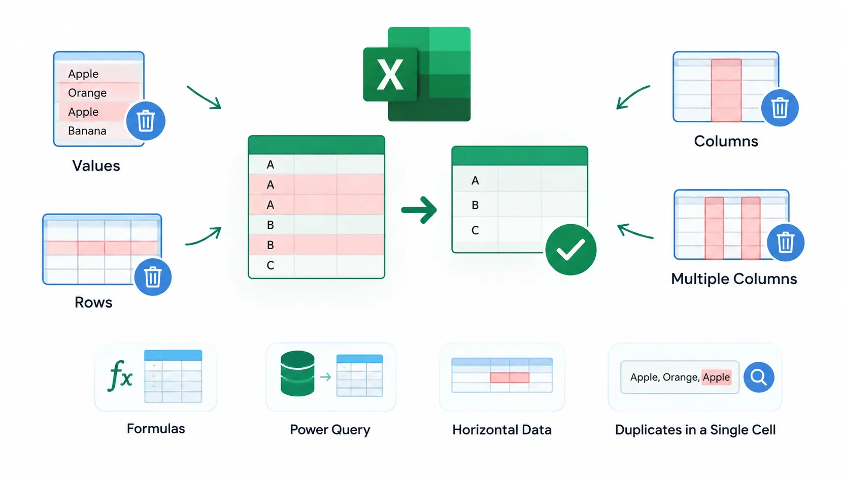
Removing duplicates sounds easy. But the right method depends on what you count as a duplicate: a repeated value, a repeated row, or a repeated record based on a few columns.
Here is the quick answer. To remove duplicates in Excel, select your data, go to Data → Remove Duplicates, tick the columns Excel should compare, and click OK. Excel keeps the first match and deletes the rest.
That covers most cases. This guide also shows you what to do when it doesn’t: multiple columns, formulas that leave your original data alone, Power Query, horizontal data, and even duplicates hiding inside a single cell.
What Does “Duplicate” Mean in Excel?
Before you delete anything, decide what “duplicate” means for your sheet. Excel will do exactly what you tell it, even if that’s the wrong thing.
Here is a small example:
| Name | Order Date | City | |
| Priya Shah | priya@example.com | 3 Jan | Pune |
| Priya Shah | priya@example.com | 3 Jan | Pune |
| Priya Shah | priya@example.com | 19 Feb | Pune |
| Rahul Mehta | priya@example.com | 5 Mar | Delhi |
Duplicate values
A single value that appears more than once in a column. “Pune” appears three times in the City column. If you only care about a list of unique cities, these are duplicates.
Duplicate rows
Two rows where every cell matches. Rows 1 and 2 above are identical in every column, so they are true duplicate rows.
Duplicate records based on selected columns
Rows that match in some columns only. Rows 1, 2, and 3 share the same Name and Email, so you might call them the same customer even though the order dates differ.
Duplicate values across multiple columns
A value that repeats across a range, such as the same product code showing up in several columns of a planning grid. This is a different problem from duplicate rows, and I cover it later.
Duplicates within a single cell
A repeated word inside one cell, like “Apple, Orange, Apple”. Excel’s built-in tool can’t see inside cells, so this needs a formula.
How to Remove Duplicates in Excel
This is the standard method. It works the same way in all modern versions of Excel for Windows and Mac. The web version has a similar command.
Step 1: Select your dataset
Click any cell inside your data. If your list has no blank rows or columns, Excel will pick up the whole range for you. For a partial list, drag to select exactly the cells you want to clean.
Step 2: Open Remove Duplicates
Go to the Data tab and click Remove Duplicates in the Data Tools group.
Step 3: Choose the columns Excel should compare
A dialog box lists your columns. Tick My data has headers if your first row is a header. Then tick only the columns that define a duplicate.
Tick every column to remove fully identical rows. Tick one column to keep one row per unique value in that column.
Step 4: Confirm the removal
Click OK. Excel deletes the duplicate rows and shows a message telling you how many it removed and how many unique values remain.
Step 5: Review the results
Don’t skip this. Scan the data and check that the count makes sense. If you started with 1,000 rows and 900 disappeared, something is probably off with the columns you ticked.
What does Excel keep when it removes duplicates?
Excel keeps the first occurrence (the one nearest the top) and deletes every later match. Two details catch people out:
- The comparison ignores the letter case, so “ANNA” and “anna” count as the same value.
- Excel compares what is displayed in the cell. A date shown as “05-Mar” is compared by that display, not by the hidden underlying value.
Because the first row wins, the order of your data decides which record survives. More on that below.
How to undo duplicate removal
Press Ctrl+Z (Cmd+Z on Mac) immediately after removing. If you’ve already saved and closed the file, the deleted rows are gone for good. That’s why a backup matters. I cover this in the “Common Mistakes” section.
How to Remove Duplicates From One Column
When you only care about one field, the choice that matters is what happens to the rest of the row.
Remove duplicate values while keeping one occurrence
Select just that column, then use Data → Remove Duplicates. Excel will warn you that it found data next to your selection. Choose Continue with the current selection only if you truly want just that column cleaned. This can break the link between the cleaned column and its neighbors, so use it on a standalone list.
Keep the entire row associated with the unique value
This is usually what you want. Select the whole table, open Remove Duplicates, then tick only the one column. Excel deletes the whole row for each repeated value, so your data stays aligned.
Remove duplicate emails
Email is the classic key for contact lists. Select all columns, tick only Email, and run the tool. Before you do, clean up stray spaces with =TRIM(B2), because “sam@example.com ” with a trailing space is not treated as a match for “sam@example.com”.
Remove duplicate names
Be careful here. Two different people can share a name. If you remove duplicates on Name alone, you may delete a real customer. Combine Name with another column such as email or phone number instead.
Remove duplicate dates
If you need a list of unique dates, copy the date column to a new sheet first, then run Remove Duplicates there. Check that all dates are true dates and not text. A date stored as text and one stored as a number look identical but won’t match.
How to Remove Duplicate Rows in Excel
Remove rows that are completely identical
Select the whole table, open Remove Duplicates, and make sure every column is ticked. Only rows that match in all columns are deleted. This is the safest option.
Remove rows based on selected columns
Tick only the columns that identify a record. Rows that match in those columns are treated as duplicates, even if other columns differ. Excel then keeps the first one.
Example: Remove duplicate customer records
Imagine a CRM export where the same customer appears three times because they signed up through different forms. The name and email match, but the signup source differs. Tick Name and Email only. You end up with one row per customer, using the top row’s signup source.
Example: Keep one customer per email address
Tick only Email. Every email now appears once. This is the cleanest way to prepare a mailing list, as long as the email is reliably filled in for every row.
How to Remove Duplicates Based on Multiple Columns
When one column isn’t enough to identify a record, you combine several. In database terms this is a composite key: a combination of fields that is unique together. You can read the idea on Wikipedia’s composite key page.
In Excel, you create a composite key by ticking more than one column in the Remove Duplicates dialog. A row is only a duplicate if all ticked columns match.
Remove duplicates based on Name + Email
Tick both. This protects you from deleting two different people who share a name, or two people sharing a family email address.
Remove duplicates based on Customer ID + Date
Useful for transaction logs where the same event was imported twice. The same customer can buy on different days, so only rows with the same ID and date are removed.
Remove duplicates based on Product + Date
This fits inventory or price lists. You keep one row per product per day, which removes accidental double entries without hiding real changes over time.
How to choose the right combination of columns
Ask one question: what makes a row unique in real life? Use this table as a guide:
| Your data | Columns that define a duplicate |
| Mailing list | |
| Customer database | Customer ID, or Name + Email |
| Sales transactions | Order ID, or Customer ID + Date + Amount |
| Daily price list | Product + Date |
| Survey responses | Respondent ID, or Email + Submission date |
| Exact copy-paste errors | All columns |
How to Find Duplicates Before Removing Them
Looking first is a habit I’d recommend to anyone. It takes a minute and prevents painful mistakes.
Highlight duplicates with Conditional Formatting
Select the column, then go to Home → Conditional Formatting → Highlight Cells Rules → Duplicate Values. Pick a color. Every repeated value lights up, including the first occurrence.
Filter duplicate values
After highlighting, use the column’s filter dropdown and choose Filter by Color. You’ll see only the duplicates, which makes it easy to inspect them.
Sort the data before removing duplicates
Sorting puts matching records next to each other. It also controls which record Excel keeps, because the top row survives.
Create a backup before permanent deletion
Right-click the sheet tab, choose Move or Copy, tick Create a copy, and click OK. Now you have a safe original to return to.
How to Remove Duplicates Without Deleting the Original Data
The Remove Duplicates button is destructive. If you want to keep your source data intact, use formulas instead. The UNIQUE function is available in Microsoft 365, Excel 2021 and later, and Excel for the web.
Use the UNIQUE function
=UNIQUE(A2:A100)
This returns a list of unique values in a new location and spills down automatically. Your original column stays untouched. One thing to know: if your range includes blank cells, the result will show a 0 for them. Wrap the range in FILTER to avoid that (see below).
Use UNIQUE with multiple columns
=UNIQUE(A2:C100)
With more than one column, UNIQUE treats each row as one item and returns unique rows. It’s the formula version of ticking all columns in Remove Duplicates.
Use FILTER with UNIQUE
=UNIQUE(FILTER(A2:A100, A2:A100<>””))
This drops blank cells first, then returns the unique values. You can also filter by a condition, for example only unique customers from one region.
Sort the unique results
=SORT(UNIQUE(A2:A100))
This gives you an alphabetical list of unique values in one formula.
When are formulas better than Remove Duplicates? Use formulas when the source data changes often, when you need to keep the original, or when you want results that update on their own. Use the button for a quick one-time cleanup.
Remove Duplicates With COUNTIF or COUNTIFS
These functions don’t remove anything. They flag duplicates so you can review and delete them yourself. They also work in older Excel versions that don’t have UNIQUE.
Identify the first occurrence
In a helper column (say B2), enter:
=COUNTIF(A2:A2,A2)
Copy it down. The first time a value appears, the result is 1. The second time, it’s 2, and so on. The trick is the range A2:A2, which expands as you copy it down.
Identify subsequent duplicates
Any row where the result is 2 or higher is a repeat. Filter the helper column for those numbers to see only the later duplicates.
Create a duplicate flag
=COUNTIF(A2:A2,A2)>1
This returns TRUE for every repeat and FALSE for the first occurrence. Filter for TRUE, review the rows, and delete them.
Use COUNTIFS for duplicate combinations
=COUNTIFS(A2:A2,A2,B2:B2,B2)>1
This flags a row only when both columns match a row above. It’s the formula version of a composite key.
How to Remove Duplicates From Multiple Columns Independently
This is a different problem from removing duplicate rows, and it’s where the standard tool falls short.
Removing duplicate rows compares entire records. Removing repeated values independently means each column gets its own clean list, regardless of what’s in the other columns.
A practical example: you have a planning sheet where columns hold dates for different projects. Several dates repeat within each column. You want each column to show every date only once, and you don’t care that the columns will end up different lengths.
Questions like this come up often on forums usually from people who tried the Remove Duplicates button and got the wrong result.
Why normal Remove Duplicates does not solve this problem
If you select several columns and run the tool, Excel treats each row as one record. A date in column A that also appears in column B is not removed, because the rows as a whole aren’t identical. And when it does delete a row, it deletes cells from every column at once.
Formula approach
Give each column its own UNIQUE formula. For column A, in a new area:
=UNIQUE(FILTER(A2:A100, A2:A100<>””))
Copy the same pattern for B, C, and so on, pointing each formula at its own column. Each column becomes a clean list. The results spill to different lengths, which is exactly what you want here.
Power Query approach
Load your table into Power Query. For each column, create a reference query, keep only that column, and use Remove Rows → Remove Duplicates. Then load each result to its own sheet or range. It takes more setup than formulas but handles large data well and can be refreshed.
When to use each approach
| Situation | Better choice |
| A few columns, Excel 365 | UNIQUE formulas |
| Many columns or a large dataset | Power Query |
| Data that changes often | Either, since both refresh |
| Older Excel without UNIQUE | Power Query |
How to Remove Duplicates From Data Arranged Horizontally
Excel’s Remove Duplicates button works on rows. If your data runs across a row, like B2:E2, it doesn’t fit the tool well.
Use TRANSPOSE + UNIQUE
=TRANSPOSE(UNIQUE(TRANSPOSE(B2:E2)))
Here’s why this works. UNIQUE compares rows by default. The inner TRANSPOSE turns your horizontal data into a vertical list, UNIQUE removes the repeats, and the outer TRANSPOSE turns the answer back into a row.
There is also a shorter route. UNIQUE has an optional argument that makes it compare columns instead:
=UNIQUE(B2:E2, TRUE)
Setting the second argument to TRUE tells Excel to compare across columns. Both formulas give the same result. The TRANSPOSE version is easier to understand at first, and the shorter one is easier to maintain.
How to Remove Duplicate Values From a Single Cell
Sometimes a single cell holds a list:
Before: Apple, Orange, Apple, Banana, Orange
After: Apple, Orange, Banana
The Remove Duplicates button can’t do this, because it only compares cells to each other.
Excel 365 formula approach
The idea is simple: split the text into pieces, remove repeats, then join the pieces back together. Excel has a function for each step.
TEXTSPLIT + UNIQUE + TEXTJOIN
=TEXTJOIN(“, “, TRUE, UNIQUE(TEXTSPLIT(A2, “, “), TRUE))
Here’s what each part does:
- TEXTSPLIT(A2, “, “) splits the cell at every comma and space, producing a horizontal list.
- UNIQUE(…, TRUE) removes repeats. The TRUE is needed because the split result runs across columns.
- TEXTJOIN(“, “, TRUE, …) stitches the unique items back into one cell.
Match the delimiter to your data. If the cell uses commas with no spaces, use “,” instead.
What to do in older Excel versions
TEXTSPLIT is only available in Microsoft 365 and Excel 2024. In older versions you have three options:
- Use Data → Text to Columns to split the cell into columns, then remove repeats manually or with a helper formula.
- Use Power Query’s Split Column by Delimiter, remove duplicates, and merge back.
- Use a short VBA macro.
How to Remove Duplicates With Power Query
Power Query is Excel’s built-in data cleaning tool. It records every step you take, so you can run the same cleanup again with one click. You can read more about it on Wikipedia’s Power Query page.
Load the data into Power Query
Click any cell in your table, then go to Data → From Table/Range. The Power Query Editor opens in a new window.
Select the columns
Click the header of the column you want to check. Hold Ctrl to select more than one. Select all columns to remove fully identical rows.
Choose Remove Rows → Remove Duplicates
On the Home tab, click Remove Rows → Remove Duplicates.
Remove duplicates based on selected columns
Power Query only compares the columns you selected before clicking the command. Select Name and Email, for instance, and it keeps the first row for each Name + Email pair.
Refresh the query later
When new data arrives, right-click the output table and choose Refresh. The same steps run again automatically.
Power Query vs Remove Duplicates
There’s one behavior difference worth knowing. Power Query treats “ANNA” and “anna” as different values, while the Excel button treats them as the same. Clean the case first with the Transform → Format → lowercase option if that matters to you.
Use Power Query when you’ll repeat the same cleanup. Use the regular button for one-off jobs.
How to Remove Duplicates From Two Excel Sheets
Sometimes the question isn’t “what repeats inside this list?” but “what appears in both lists?”
Compare two lists
Put both lists side by side or on separate sheets. Decide which column holds the matching value, such as an email or ID.
Find matching records
In a helper column next to List 1, use:
=COUNTIF(Sheet2!A2:A500, A2)>0
TRUE means the value also exists in Sheet 2.
Return only unique records
To keep only the records from List 1 that are not in List 2, use FILTER in Excel 365:
=FILTER(A2:A500, COUNTIF(Sheet2!A2:A500, A2:A500)=0)
In older versions, filter your helper column for FALSE and copy the results.
Use Power Query for recurring comparisons
If you compare the same two lists every week, use Power Query’s Merge Queries with a Left Anti join. It returns rows from the first table that have no match in the second, and it refreshes with one click.
How to Remove Duplicates While Keeping the Newest or Oldest Record
This comes up constantly. Say a customer has updated their details five times, and you want only the latest record.
Excel always keeps the first row it finds. So you control the outcome by sorting first.
Sort by date first
Select your table and go to Data → Sort. Sort by the date column. Choose Newest to Oldest to keep the latest record, or Oldest to Newest to keep the earliest.
Remove duplicates after sorting
Now run Data → Remove Duplicates and tick only the column that identifies the record, such as Customer ID. Excel keeps the top row for each customer, which is the one you sorted to the top.
Example: Keep the latest customer record
Sort by Last Updated, newest first. Run Remove Duplicates on Customer ID. Each customer now has only their most recent entry.
Example: Keep the earliest transaction
Sort by Transaction Date, oldest first. Run Remove Duplicates on Customer ID. Each customer shows only their first purchase, which helps with cohort or retention analysis.
If you skip the sort, Excel keeps whichever row happens to be on top. That can silently discard the record you wanted.
How to Remove Duplicates in an Excel Table
If your data is formatted as an Excel Table (Ctrl+T), you have a second route to the same tool.
Use Table Design → Remove Duplicates
Click inside the table. A Table Design tab appears on the ribbon. Click Remove Duplicates in the Tools group.
Select the fields that define uniqueness
The dialog works the same way as the Data tab version. Tick the columns that define a duplicate and click OK.
Preserve structured data
Tables resize automatically, and formulas that reference them stay intact. Deleting rows from a table also avoids leaving gaps, so it’s a tidier option for data you plan to keep building on.
Remove Duplicates in Different Excel Versions
The basic button exists in every modern version. What changes is which formulas you can use.
Microsoft 365 / Excel for the web
You get everything: Remove Duplicates, UNIQUE, FILTER, SORT, TEXTSPLIT, Power Query, and Office Scripts (in supported plans).
Excel 2021
UNIQUE, FILTER, and SORT are available. TEXTSPLIT is not.
Excel 2019
No dynamic array functions such as UNIQUE. Use Remove Duplicates, COUNTIF/COUNTIFS, and Power Query. TEXTJOIN is available.
Excel 2016
Power Query is built in under Data → Get & Transform. UNIQUE is not available, and TEXTJOIN is generally limited to subscription versions.
Excel 2010 and earlier
Remove Duplicates is available from Excel 2007 onward. For Excel 2010, Power Query can be installed as a free Microsoft add-in. Otherwise, rely on COUNTIF helper columns and the Advanced Filter’s “Unique records only” option.
A good rule: if a formula spills into several cells on its own, it needs a modern version of Excel. Otherwise, assume it will work in older ones.
Remove Duplicates With VBA or Office Scripts
When automation makes sense
Use automation when you clean the same file layout every day or week and want to skip the clicking. If you’re cleaning once, don’t bother.
VBA for recurring cleanup
Here is a short macro that removes duplicates based on the first two columns of a range:
Sub RemoveDupes()
Range(“A1:D1000”).RemoveDuplicates Columns:=Array(1, 2), Header:=xlYes
End Sub
The Columns:=Array(1, 2) part tells Excel to compare columns 1 and 2. Change the range and column numbers to fit your sheet.
Office Scripts for Microsoft 365
Office Scripts do the same job in Excel for the web using TypeScript, and they can be run from Power Automate. They are useful when the cleanup is part of a larger online workflow.
When Power Query is a better choice
For most people, Power Query is easier than writing code and handles recurring cleanup just as well. Reach for VBA or Office Scripts only when you need to trigger the job automatically or combine it with other actions.
Common Mistakes When Removing Duplicates in Excel
I’ve seen each of these cause real data loss.
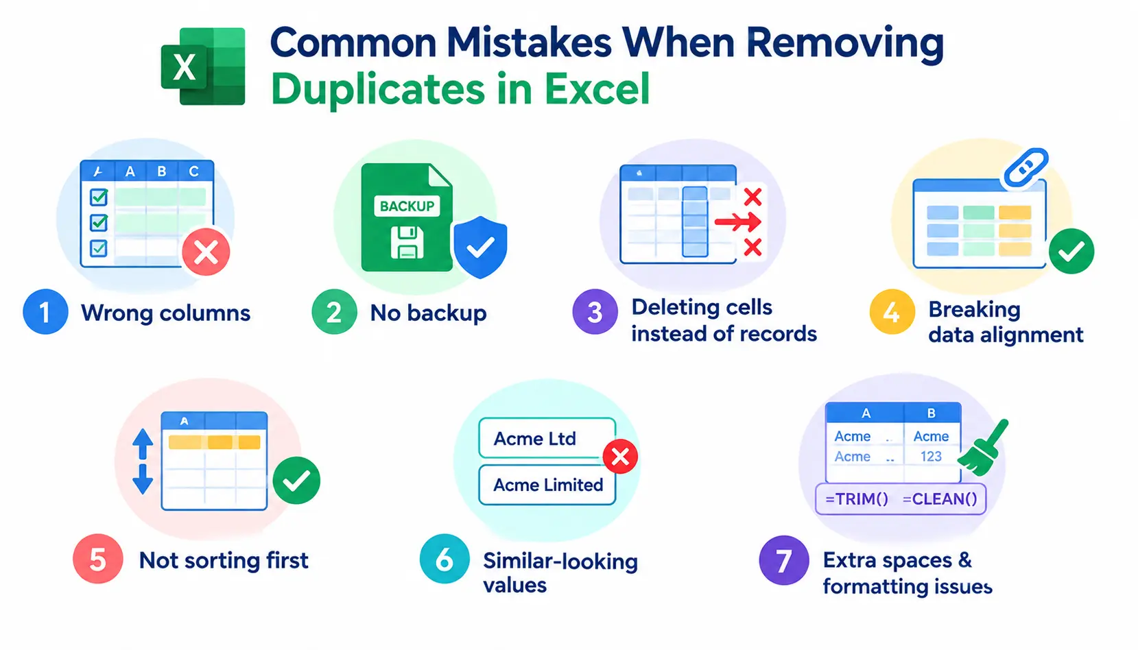
Selecting the wrong columns
Tick too many columns and nothing is removed. Tick too few and you delete real records. Re-read the dialog before clicking OK.
Removing duplicates before creating a backup
Undo only works until you close the file. Save a copy first.
Deleting duplicate cells instead of records
Cleaning one column inside a larger table can push values out of alignment with their neighbors. Select the whole table unless you really only want that column.
Forgetting that associated data must stay aligned
If you sort one column on its own, its values no longer match the rest of the row. Always sort the full table.
Not sorting before choosing which record to keep
Excel keeps the top row. If you need the newest, largest, or most complete record, sort first.
Treating similar-looking values as identical
“Acme Ltd” and “Acme Limited” look alike to you but not to Excel. The tool only matches exact text.
Not checking spaces and inconsistent formatting
Extra spaces, non-breaking spaces, and text-formatted numbers all block matches. Use =TRIM() and =CLEAN() on messy data before removing duplicates.
Excel Remove Duplicates: Which Method Should You Use?
Use this table to pick the right approach quickly.
| Situation | Best method |
| Delete duplicate rows once | Remove Duplicates |
| Find duplicates first | Conditional Formatting |
| Create a unique list | UNIQUE |
| Flag duplicates | COUNTIF |
| Duplicate combinations | COUNTIFS |
| Repeated data cleaning | Power Query |
| Horizontal duplicates | TRANSPOSE + UNIQUE |
| Duplicates inside cells | TEXTSPLIT + UNIQUE + TEXTJOIN |
| Automated cleanup | VBA / Office Scripts |
Frequently Asked Questions
1. How do I remove duplicates in Excel but keep one?
Select your data, go to Data → Remove Duplicates, choose the columns to compare, and click OK. Excel automatically keeps the first occurrence of each duplicate and deletes the others.
2. How do I remove duplicates from one column without deleting the entire row?
Copy the column to a new location and run Remove Duplicates there. Alternatively, use =UNIQUE() to create a clean list without touching the original data.
3. How do I remove duplicate rows in Excel?
Select the whole table, open Data → Remove Duplicates, and tick all columns. Only rows that match in every column are removed.
4. How do I remove duplicates based on two columns?
In the Remove Duplicates dialog, tick only those two columns. A row is deleted only when both values match a row above it.
5. How do I remove duplicates without affecting adjacent columns?
Select only the column you want to clean and choose Continue with the current selection when Excel warns you. Be aware this can misalign data, so a safer option is to extract the unique list with UNIQUE in another location.
6. How do I find duplicates before deleting them?
Use Home → Conditional Formatting → Highlight Cells Rules → Duplicate Values. Duplicates are highlighted so you can review them first.
7. What is the difference between UNIQUE and Remove Duplicates?
Remove Duplicates permanently deletes rows from your original data. UNIQUE is a formula that creates a separate list of unique values and leaves the source intact. UNIQUE also updates automatically when the data changes.
8. How do I remove duplicates from multiple columns separately?
Apply a separate UNIQUE formula to each column, or use Power Query to create one cleaned query per column. The standard Remove Duplicates button can’t do this because it compares entire rows.
9. How do I remove duplicates from a single cell?
In Microsoft 365, use =TEXTJOIN(“, “, TRUE, UNIQUE(TEXTSPLIT(A2, “, “), TRUE)). In older versions, split the cell with Text to Columns or Power Query first.
10. How do I remove duplicates in Excel automatically?
Use Power Query and refresh it when your data changes. For fully automatic runs, use a VBA macro or an Office Script.
Conclusion
To remove duplicates in Excel the simple way, use Data → Remove Duplicates and tick the right columns. For anything more complex, such as keeping your original data, comparing combinations, or cleaning repeatedly, formulas and Power Query give you more control.
Before you delete anything, back up your file, check for stray spaces, and decide what a duplicate means for your data. Those three habits prevent most mistakes.
If you get stuck on an unusual layout, the excel community is a good place to ask, and Microsoft’s official Excel support pages document each function mentioned here.