
If you have ever wondered how computing began before smartphones, laptops, or even the microchip, the story starts with first generation computers. These machines were massive, hot, and slow by today’s standards. Yet they laid the foundation for every device we use now.
This guide walks through what first generation computers were, how they worked, why they mattered, and why they eventually disappeared. Whether you are a student preparing notes for an exam or someone simply curious about computing history, you will find a complete and practical explanation here.
What Are First Generation Computers?
First generation computers were the earliest electronic computers, built using vacuum tubes as their primary switching and amplifying components. They ran on machine language, the most basic form of programming, and relied on punch cards or paper tape for input.
Think of a vacuum tube as an early version of a switch that could turn an electrical signal on or off, similar to how a transistor works in modern chips, except far bigger, far hotter, and far less reliable. A single first generation computer could contain thousands of these tubes.
Why They Are Called the First Generation
Computer history is usually divided into generations based on the core technology used to build the hardware. The first generation earns its name simply because it came first: it used vacuum tube technology before transistors, integrated circuits, and microprocessors took over in later generations.
Each generation solved the biggest problem of the one before it. That pattern becomes clearer as you read through this article.
Time Period (1940 to 1956)
Most historians place the first generation of computers between roughly 1940 and 1956. This window covers the development of early wartime calculating machines through to the first commercially available computers sold to businesses and government agencies.
History of First Generation Computers
Computing Before Electronic Computers
Long before vacuum tubes, people relied on mechanical devices to calculate. Charles Babbage designed the Analytical Engine in the 1830s, a mechanical device widely regarded as a conceptual ancestor of the modern computer. Ada Lovelace, who worked closely with Babbage, is often credited with writing what many consider the first algorithm intended for a machine, according to Wikipedia.
By the 1930s and early 1940s, electromechanical machines using relays and switches began to appear. Howard Aiken’s Harvard Mark I, built with support from IBM, is a good example of this transitional stage between mechanical and electronic computing.
The Birth of Electronic Computing
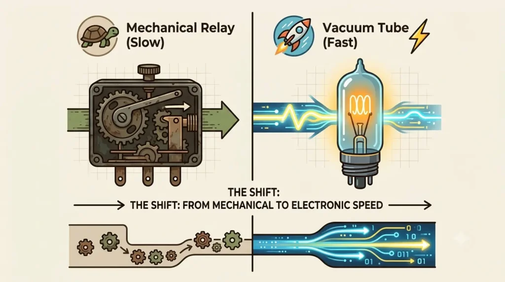
The real shift happened when engineers replaced mechanical relays with vacuum tubes. Tubes could switch on and off thousands of times faster than any mechanical part, which meant computers could finally process information at electronic speed instead of mechanical speed.
This shift is what separates true first generation computers from the electromechanical machines that came before them.
Role of World War II in Computer Development
War pushed computing forward faster than peacetime research ever could. Military forces needed rapid calculations for artillery firing tables, code breaking, and logistics. Alan Turing’s work on codebreaking machines in Britain and the U.S. Army’s funding of ENIAC for artillery calculations both came directly out of wartime necessity.
Without that urgency, historians generally agree electronic computing would have developed much more slowly.
How First Generation Computers Worked
Vacuum Tube Technology
A vacuum tube is a sealed glass device that controls electric current in an enclosed vacuum. Inside, a heated filament releases electrons that flow toward a metal plate, and by controlling that flow, engineers could use tubes to amplify signals or act as on-off switches, the same basic function a transistor performs today.
The problem was scale and durability. A single computer needed thousands of tubes, and tubes generated intense heat, burned out often, and consumed enormous amounts of electricity. Technicians sometimes spent hours each day just replacing burnt-out tubes before the machine could even run.
Machine Language
First generation computers understood only machine language, which is a series of 0s and 1s that directly corresponds to the computer’s hardware instructions. There was no user-friendly programming language yet.
Programming meant physically rewiring circuits or manually feeding binary instructions, a process that could take days for a single task. This is one reason these machines were used mostly by trained specialists rather than everyday operators.
Magnetic Drum Memory
Early computers stored data on magnetic drums, which were rotating cylinders coated with magnetic material. Data was written and read as the drum spun past a read-write head, similar in concept to how a record player needle interacts with a vinyl disc.
Drum memory was slow compared to modern storage, but it was a major improvement over earlier storage methods and became a standard feature in machines like the IBM 650.
Punch Cards and Paper Tape
Input and output relied heavily on punch cards and paper tape. Operators encoded data and instructions as patterns of holes, and the machine read these patterns to execute commands or store results.
This method traced back to Herman Hollerith’s tabulating machines from the 1890s census, showing how punch card technology carried over from earlier data processing systems into the first computer generation.
Stored Program Concept
One of the most important ideas of this era came from mathematician John von Neumann, who proposed that a computer’s instructions could be stored in memory alongside its data, rather than being hardwired for each task. This is known as the stored program concept, and it is described in detail on Wikipedia’s Von Neumann architecture page.
EDVAC was one of the first machines designed around this idea. It meant a computer could be reprogrammed for a new task without physically rewiring it, a breakthrough that shaped every computer built afterward.
Characteristics of First Generation Computers
Large Size
These computers were enormous. ENIAC, for example, occupied a room roughly 1,800 square feet and weighed around 30 tons. Entire buildings were sometimes needed just to house one machine.
High Power Consumption
Running thousands of vacuum tubes demanded a huge amount of electricity. ENIAC alone consumed around 150 kilowatts of power, enough to dim the lights in the surrounding neighborhood when it started up, according to widely cited historical accounts.
Heat Generation
All that power consumption produced enormous heat. Facilities needed dedicated cooling systems just to prevent the tubes from failing even faster than they already did.
Limited Speed
By today’s standards, these machines were painfully slow, capable of only a few thousand calculations per second. A basic modern smartphone processes billions of operations per second, which puts the gap in perspective.
Low Storage Capacity
Memory was extremely limited, often just a few kilobytes. Complex programs had to be broken into small chunks that could fit within these tight constraints.
Reliability Issues
Vacuum tubes failed constantly. It was common for a machine to run for only a few hours before a tube burnt out and had to be located and replaced, which made long, uninterrupted computing sessions a real challenge.
Expensive Operation
Between the cost of electricity, cooling, replacement parts, and specialized staff, running one of these computers was extremely expensive. Only governments, universities, and large corporations could afford them.
Features of First Generation Computers
- Built using vacuum tube technology for switching and amplification
- Programmed using machine language (binary code)
- Used magnetic drums and punch cards for memory and input/output
- Extremely large physical size, often filling entire rooms
- Operated by trained specialists, not general users
- Generated significant heat and required constant maintenance
- Represented the first practical application of the stored program concept
Advantages of First Generation Computers
First generation computers may look primitive now, but they were revolutionary for their time.
- They made electronic calculation possible at speeds no mechanical device could match
- They proved the stored program concept, which remains the foundation of computing today
- They enabled complex scientific and military calculations that were previously impossible by hand
- They opened the door to automation in fields like census processing and scientific research
- They laid the technical groundwork that made second generation computers possible
Disadvantages of First Generation Computers
The limitations of these machines were significant and directly shaped what came next.
- Extremely large size made them impractical for most organizations
- High power consumption made them expensive to operate
- Excessive heat generation caused frequent hardware failures
- Vacuum tubes were unreliable and needed constant replacement
- Machine language programming was slow and required deep technical expertise
- Very limited memory restricted the complexity of programs they could run
- High cost limited access to governments, universities, and large corporations only
Examples of First Generation Computers
1. ENIAC
Year: 1945 (completed), unveiled publicly in 1946 Developers: J. Presper Eckert and John Mauchly Where: University of Pennsylvania
Features
ENIAC, short for Electronic Numerical Integrator and Computer, is widely considered the first general purpose electronic digital computer. It used around 18,000 vacuum tubes and could perform thousands of additions per second.
Applications
It was originally built to calculate artillery firing tables for the U.S. Army, though it also contributed to early hydrogen bomb calculations.
Historical Importance
ENIAC proved that large-scale electronic computing was possible, and it directly influenced the design of every computer that followed it. You can read more background on its Wikipedia page.
2. EDVAC
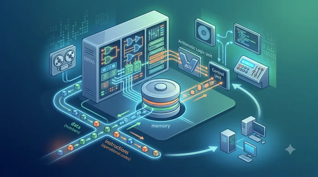
Built by the same Eckert and Mauchly team with input from John von Neumann, EDVAC (Electronic Discrete Variable Automatic Computer) introduced the stored program concept in a practical design. It was completed around 1949 and became a model for future computer architecture.
3. EDSAC
Developed at Cambridge University under Maurice Wilkes and completed in 1949, EDSAC (Electronic Delay Storage Automatic Calculator) was one of the first computers to actually run stored programs successfully, putting von Neumann’s theory into working practice.
4. UNIVAC I
Released in 1951 by the Eckert-Mauchly Computer Corporation, later part of Remington Rand, UNIVAC I became the first commercially produced computer in the United States. It gained public fame after correctly predicting the outcome of the 1952 U.S. presidential election on live television.
5. IBM 701
Launched in 1952 and 1953, the IBM 701 was IBM’s first commercial scientific computer. It marked IBM’s serious entry into the computer business and was used mainly for scientific and engineering calculations by government and research organizations.
6. IBM 650
Introduced in 1954, the IBM 650 used magnetic drum memory and became one of the best-selling computers of its era, with hundreds of units installed at businesses and universities. Its relative affordability, compared to other machines of the time, helped bring computing to a wider range of organizations.
READ MORE ON Examples of First Generation Computers
Applications of First Generation Computers
Scientific Research
Universities and research labs used these computers for complex mathematical modeling, including early work in nuclear physics.
Military Operations
Militaries used them for code breaking, ballistic calculations, and logistics planning, tasks that were previously done manually and slowly.
Census Processing
UNIVAC I and its successors were used by the U.S. Census Bureau to process population data far faster than manual tabulation ever allowed.
Weather Forecasting
Early meteorologists used these machines to run basic numerical weather models, a practice that eventually grew into the sophisticated forecasting systems used today.
Business Data Processing
Large corporations began adopting machines like the IBM 650 for payroll, inventory, and accounting tasks, marking the start of computers entering everyday business operations.
Why First Generation Computers Were Replaced
Major Limitations
The combination of size, heat, cost, and unreliability made first generation computers difficult to scale. Businesses and researchers needed something smaller, cheaper, and far more dependable.
Rise of Transistor Technology
Bell Labs researchers invented the transistor in 1947, and by the mid-1950s it started replacing vacuum tubes in computer design. Transistors were smaller, generated far less heat, consumed less power, and lasted much longer than vacuum tubes.
Transition to Second Generation Computers
By 1956, computers built with transistors began appearing, marking the start of the second generation. This shift solved most of the core problems that had limited the first generation, paving the way for smaller, faster, and more affordable machines.
First Generation vs Second Generation Computers
Comparison Table
| Feature | First Generation | Second Generation |
|---|---|---|
| Core Technology | Vacuum tubes | Transistors |
| Time Period | 1940 to 1956 | 1956 to 1963 |
| Size | Very large, room-sized | Smaller, more compact |
| Power Consumption | Very high | Reduced significantly |
| Heat Generation | Excessive | Much lower |
| Reliability | Frequent hardware failures | Far more reliable |
| Programming | Machine language | Assembly language and early high-level languages |
| Cost | Extremely expensive | More affordable, wider adoption |
Key Differences
The biggest difference comes down to the core switching component. Vacuum tubes gave way to transistors, and that single change solved most of the size, heat, and reliability problems that defined the first generation.
Programming also became more practical during the second generation, as assembly language and early high-level languages like FORTRAN began replacing pure machine code.
Legacy of First Generation Computers
Impact on Modern Computing
Every computer built since 1956 owes something to this first generation. The stored program concept introduced through EDVAC and proven in EDSAC still forms the basic architecture of the device you are using to read this article right now.
Technologies That Continued to Evolve
Magnetic storage evolved into hard drives. Punch card input evolved into keyboards and digital interfaces. Machine language evolved into the layered programming languages developers use today.
Lessons from the First Generation
Perhaps the biggest lesson is that raw computing power always comes with tradeoffs. Engineers of that era learned that speed alone was not enough. Reliability, cost, and usability mattered just as much, and that lesson continues to shape hardware design decisions today.
If you want to see how enthusiasts and historians still discuss these early machines, communities like the r/computing subreddit and various computer history groups on LinkedIn regularly share restoration projects and archival photos of vacuum tube era hardware.
Conclusion
First generation computers were far from perfect. They were massive, power-hungry, and unreliable by any modern measure. But they proved something that no one had proven at scale before: that electronic computing was possible, and that a stored program could control a machine’s behavior.
Without the vacuum tube era, there would be no transistor era, no microprocessor, and no laptop or phone in your hand today. Understanding first generation computers is not just an academic exercise. It is understanding the very first step in a chain of innovation that never stopped moving forward.
Frequently Asked Questions About First Generation Computers
What are first-generation computers?
First generation computers are the earliest electronic computers, built between roughly 1940 and 1956, using vacuum tubes for processing and switching.
When were first-generation computers used?
They were used mainly between 1940 and 1956, before transistor technology replaced vacuum tubes and started the second generation.
Why are they called first-generation computers?
They are called the first generation because they were the earliest electronic computers, built before transistors, integrated circuits, and microprocessors existed.
What technology was used in first-generation computers?
They used vacuum tube technology for processing, magnetic drums for memory, and punch cards or paper tape for input and output.
What is a vacuum tube in a computer?
A vacuum tube is a sealed glass device that controls the flow of electrons to amplify or switch electrical signals, functioning similarly to how a transistor works in modern electronics.
What are the characteristics of first-generation computers?
They were large, expensive, power-hungry, and unreliable, generating excessive heat and offering very limited memory and processing speed compared to later machines.
What are the advantages of first-generation computers?
They proved that electronic computing was viable, enabled complex calculations previously impossible by hand, and introduced the stored program concept that still underlies modern computing.
What are the disadvantages of first-generation computers?
Their major drawbacks included massive size, high power consumption, poor reliability, limited memory, and extremely high operating costs.
Which computers belong to the first generation?
Notable examples include ENIAC, EDVAC, EDSAC, UNIVAC I, IBM 701, and IBM 650.
What is ENIAC?
ENIAC was one of the first general purpose electronic digital computers, built in 1945 at the University of Pennsylvania to calculate artillery firing tables for the U.S. Army.
What is UNIVAC I?
UNIVAC I was the first commercially produced computer in the United States, released in 1951 and famous for predicting the 1952 presidential election on live television.
What is EDVAC?
EDVAC was a computer designed around the stored program concept proposed by John von Neumann, completed around 1949 and highly influential on future computer architecture.
What programming language did first-generation computers use?
They used machine language, a low-level binary code that directly corresponded to hardware instructions, since higher-level programming languages had not yet been developed.
Why were first-generation computers replaced?
They were replaced because transistors, invented at Bell Labs in 1947, offered a smaller, cooler, more reliable, and cheaper alternative to vacuum tubes, starting the second generation around 1956.
What is the difference between first- and second-generation computers?
First generation computers used vacuum tubes and were large, hot, and unreliable, while second generation computers used transistors, making them smaller, more efficient, and considerably more dependable.