
Long before smartphones, laptops, or even desktop PCs, a handful of enormous, room-filling machines quietly changed the course of human history. The examples of first generation computers built between 1940 and 1956 represent the true beginning of the digital age, the moment humanity first taught electricity to think. These machines were not sleek or portable.
They weighed tens of thousands of kilograms, consumed enough power to light entire city blocks, and had to be programmed by physically rearranging wires and switches. Yet they performed calculations that no human team could match in speed or accuracy.
The most famous examples of first generation computers include ENIAC, the first general-purpose electronic computer; UNIVAC I, the first commercial computer; IBM 701, which launched one of the greatest technology companies into the computing era; EDVAC, which introduced the stored program concept that underlies every modern computer; and several other pioneering machines that each contributed a critical piece to the puzzle of modern computing.
In this blog, we will explore every major example of first generation computers in detail. For each machine, we will cover when it was built, who built it, what made it unique, what it was used for, and why it matters. We will also examine the shared characteristics of all first generation computers, their advantages and disadvantages, how they compare to second generation machines, and answer the most frequently asked questions about these historic devices. Whether you are a student, an educator, or simply curious about computing history, this guide will give you a complete picture of where the digital world began.
What Is a First Generation Computer?
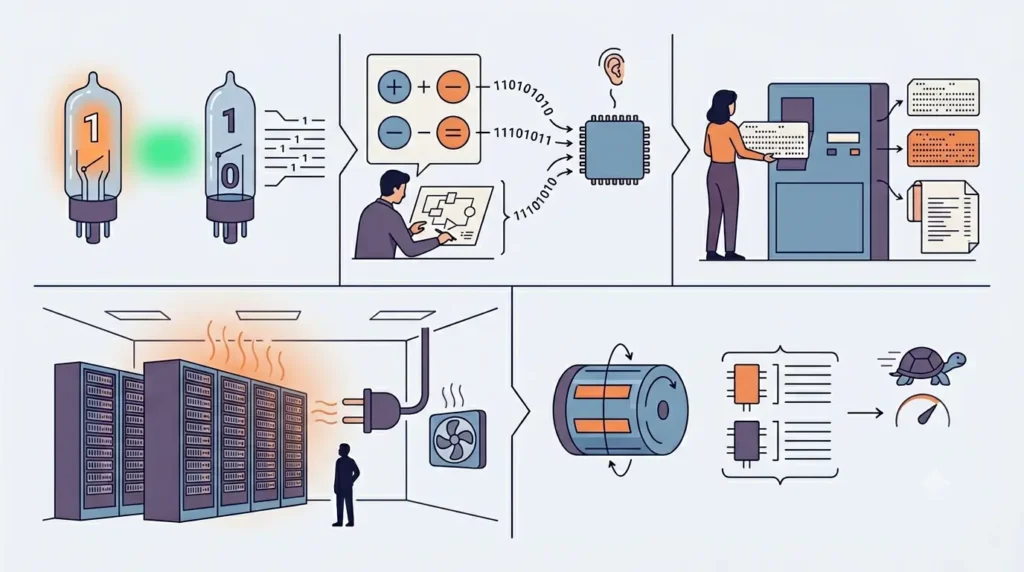
A first generation computer is any electronic computing machine built during the period from approximately 1940 to 1956 that used vacuum tubes as its primary electronic switching technology. Vacuum tubes are glass cylinders that control the flow of electric current and act as the on/off switches that represent binary 1s and 0s in digital logic. Because each vacuum tube is roughly the size of a light bulb, computers built from thousands of them were inevitably enormous.
These machines were programmed using machine language, the lowest level of computer programming consisting entirely of binary instructions directly understood by the hardware. There were no programming languages, no operating systems, and no graphical interfaces. Operators communicated with the computer through punch cards, paper tape, and banks of physical switches. Output was delivered via punch cards, paper printouts, or teleprinters.
First generation computers were expensive to build and operate, required teams of engineers and technicians to maintain, generated vast amounts of heat requiring industrial cooling systems, and suffered from frequent failures of their thousands of vacuum tubes.
Despite all these limitations, they represented a revolutionary leap forward, demonstrating for the first time that electronic machines could perform complex mathematical and logical operations at speeds far beyond human capability. They paved the way for every subsequent generation of computers and laid the intellectual and engineering foundations of the modern digital world.
Key Characteristics of First Generation Computers
Before examining individual examples, it helps to understand the defining features that all first generation computers share. These characteristics set them apart from every later generation and explain both their capabilities and their limitations.
1. Use of Vacuum Tubes
Vacuum tubes were the core logic component of every first generation computer. Each tube functions as an electronic switch that can be either on (representing 1) or off (representing 0), enabling binary digital computation.
A single computer might contain anywhere from a few thousand to over eighteen thousand vacuum tubes. While groundbreaking, vacuum tubes were bulky, expensive, and fragile. They generated enormous heat, burned out regularly, and had to be replaced frequently, making maintenance a constant and demanding task.
2. Machine Language Programming
First generation computers were programmed entirely in machine language, sequences of binary numbers that directly instructed the hardware to perform specific operations. There were no compilers, no assemblers, and no higher-level programming languages.
Writing a program meant understanding the exact binary instruction set of the specific machine and encoding every operation manually. This made programming extremely time-consuming, error-prone, and accessible only to highly trained specialists.
3. Punch Card Input and Output
Data was fed into first generation computers primarily through punch cards, stiff paper cards with holes punched in specific positions to represent data or instructions. Results were typically output through a card punch that produced new punch cards, or through a printer that produced paper output. Some machines used paper tape rather than punch cards. These input and output methods were slow and cumbersome by modern standards but were the most practical options available with the technology of the era.
4. Large Size and High Power Consumption
The sheer number of vacuum tubes required to build a functional computer meant that first generation machines occupied enormous physical spaces. ENIAC, for example, filled an entire room, weighed approximately thirty tons, and stretched across a wall over twenty meters long. The power consumption of these machines was equally extreme.
ENIAC consumed around 150 kilowatts of electricity during operation, enough to power a small neighbourhood. This massive power draw generated equally massive heat, requiring industrial-scale cooling infrastructure.
5. Limited Storage and Processing Speed
By modern standards, the storage and processing capabilities of first generation computers were extremely limited. Most used either electrostatic storage tubes or magnetic drum memory, which could hold only a few thousand words of data. Processing speeds, while fast compared to human calculation, were a small fraction of even the cheapest modern processor.
ENIAC could perform around five thousand additions per second, a figure that a modern smartphone processor exceeds by a factor of billions. Despite these limitations, first generation computers were astonishing achievements for their time.
List of Examples of First Generation Computers
The following are the most significant examples of first generation computers. Each represents a major milestone in computing history and contributed something unique to the development of digital technology. The table below provides a quick reference before we explore each machine in detail.
| Computer Name | Year | Developed By | Primary Use |
| ENIAC | 1945 | Mauchly & Eckert, Univ. of Pennsylvania | Military ballistics calculations |
| UNIVAC I | 1951 | Eckert-Mauchly Computer Corp. | Commercial data processing |
| IBM 701 | 1952 | International Business Machines (IBM) | Scientific and defense research |
| IBM 650 | 1953 | International Business Machines (IBM) | Business and education |
| EDVAC | 1949 | Mauchly & Eckert, Univ. of Pennsylvania | Scientific research |
| EDSAC | 1949 | Maurice Wilkes, Univ. of Cambridge | Academic research |
| LEO I | 1951 | J. Lyons & Co., United Kingdom | Business operations |
| MANIAC | 1952 | Los Alamos Scientific Laboratory | Nuclear and scientific research |
| IAS Computer | 1952 | John von Neumann, Princeton | Scientific computing |
| Harvard Mark I | 1944 | Howard Aiken, Harvard University | Mathematical calculations |
Detailed Examples of First Generation Computers
Now let us examine each of these historic machines in depth, covering their origins, technical specifications, purposes, and lasting significance.
1. ENIAC (Electronic Numerical Integrator and Computer)
ENIAC is widely regarded as the first general-purpose electronic digital computer ever built. It was designed and constructed by John Mauchly and J. Presper Eckert at the Moore School of Electrical Engineering at the University of Pennsylvania, funded by the United States Army. Construction began in 1943 and the machine became fully operational in 1945, though it was not publicly announced until 1946.
ENIAC was a machine of staggering scale. It contained approximately 18,000 vacuum tubes, 70,000 resistors, 10,000 capacitors, and 6,000 manual switches.
The entire system occupied about 167 square meters of floor space, weighed roughly 30 tons, and consumed around 150 kilowatts of electricity during operation. It could perform approximately 5,000 additions or 360 multiplications per second, making it hundreds of times faster than any electromechanical computer that preceded it.
- Technology: Vacuum tubes for all logic operations
- Speed: 5,000 additions per second
- Input/Output: IBM punch cards
- Memory: No internal stored memory; programs set via switches and patch cables
- Power consumption: Approximately 150 kilowatts
- Weight: Approximately 30 tons
ENIAC was originally designed to calculate artillery firing tables for the U.S. Army’s Ballistic Research Laboratory. Before ENIAC, these tables were calculated by teams of human computers (people doing calculations) and took months. ENIAC could produce the same results in hours.
After the war, ENIAC was used for a wide range of scientific calculations, including weather prediction studies, cosmic ray analysis, and early work related to the hydrogen bomb.
The historical significance of ENIAC cannot be overstated. It demonstrated conclusively that electronic digital computers were practical, capable, and vastly faster than any mechanical or human alternative. Every subsequent computer development builds on the foundation that ENIAC proved was possible.
2. UNIVAC I (Universal Automatic Computer I)
UNIVAC I, the Universal Automatic Computer I, holds the distinction of being the first commercially produced computer in the United States. It was developed by John Mauchly and J. Presper Eckert, the same duo who created ENIAC, this time through their own company which was eventually acquired by Remington Rand. The first UNIVAC I was delivered to the United States Census Bureau in 1951.
Unlike ENIAC, which was designed as a scientific instrument for a specific military application, UNIVAC I was designed from the outset for general commercial data processing. It was built to handle the kinds of large-scale data management tasks that businesses and government agencies needed: processing payroll, managing inventory records, performing statistical analysis, and handling the enormous data requirements of the national census.
- Technology: Vacuum tubes, approximately 5,200
- Storage: Magnetic tape for data storage and input, capable of storing around 1,000 words in internal memory
- Speed: Could process approximately 1,000 calculations per second
- Input: Magnetic tape and punch cards
- Output: Magnetic tape and high-speed printer
- Innovation: Could handle both alphabetic and numeric data
UNIVAC I became famous far beyond the technical community when CBS News used it to predict the outcome of the 1952 United States Presidential Election. Based on early returns, the computer predicted an Eisenhower landslide when most political analysts expected a close race.
The analysts initially doubted the prediction and adjusted the results before broadcasting them, but UNIVAC I turned out to be correct. The moment brought the concept of computers to millions of ordinary Americans and transformed public awareness of computing technology.
A total of 46 UNIVAC I systems were sold between 1951 and 1958, making it the first computer model produced in significant commercial quantities. Its customers included government agencies, major corporations, and research institutions, establishing the commercial computer industry as a genuine business sector.
3. IBM 701
The IBM 701, formally named the IBM Defense Calculator, was introduced in April 1952 and marked IBM’s entry into the electronic stored-program computer market.
IBM had been a dominant force in punch card tabulating machines for decades, but the 701 represented its first serious foray into electronic digital computing. It was designed primarily for scientific and defence applications and was aimed at government agencies, research laboratories, and defence contractors.
The 701 was significantly more capable than earlier machines in several respects. It was designed as a commercial product with reliability and serviceability in mind, not just as a one-off research prototype. IBM sold nineteen 701 systems between 1952 and 1956, primarily to defence contractors and research institutions working on Cold War-era projects including nuclear weapons design and aeronautical research.
- Technology: Vacuum tubes for all logic circuits
- Speed: Approximately 16,000 additions per second
- Memory: Electrostatic storage tubes, later magnetic core
- Input/Output: Punch cards and magnetic tape
- Programming: Machine language
- Notable customers: Los Alamos, Livermore National Laboratory, Boeing, Douglas Aircraft, North American Aviation
The IBM 701 is historically significant for several reasons beyond its technical specifications. It established IBM as a major player in electronic computing, launching a trajectory that would make IBM the dominant force in computing for the next three decades.
The engineering expertise IBM developed while building the 701 fed directly into subsequent models including the IBM 702, 704, and 709, each of which advanced the state of the art considerably.
4. IBM 650
The IBM 650 Magnetic Drum Data Processing Machine, introduced in 1953, became the most commercially successful first generation computer. While machines like ENIAC and IBM 701 were massive, expensive, and accessible only to the largest organisations, the IBM 650 was designed to be more compact, more affordable, and more practical for a wider range of customers.
IBM priced it at around $200,000 to purchase or $3,200 per month to lease, which, while still expensive, put it within reach of universities, medium-sized businesses, and government agencies.
The 650 used a magnetic drum as its primary memory, which was more reliable and more cost-effective than the electrostatic storage tubes used in earlier machines. Its relatively modest size, about the footprint of a large desk and some cabinets, made it practical to install in standard office and laboratory environments without requiring the specially constructed rooms needed for earlier machines.
- Technology: Vacuum tubes plus magnetic drum memory
- Storage: Magnetic drum holding 2,000 ten-digit words
- Speed: 12,500 additions per second
- Input/Output: Punch cards
- Weight: Approximately 900 kg, far lighter than predecessors
- Units sold: Over 2,000, making it the first mass-produced computer
The IBM 650 had a profound impact on computing education. IBM offered it to universities at significant discounts, and by the late 1950s hundreds of universities around the world had 650 systems that students could use to learn programming and computer science.
Many of the pioneers of the next generation of computing, the people who would go on to design the software and hardware of the 1960s and 1970s, learned their craft on IBM 650 systems. In this sense, the 650 shaped the trajectory of the entire computing profession.
5. EDVAC (Electronic Discrete Variable Automatic Computer)
EDVAC, the Electronic Discrete Variable Automatic Computer, was developed at the University of Pennsylvania by the same team responsible for ENIAC, led by Mauchly and Eckert, with crucial theoretical contributions from the mathematician John von Neumann. Work on EDVAC began in 1944 while ENIAC was still under construction, and the machine became fully operational in 1949.
EDVAC represents one of the most intellectually significant advances in computing history because it was the first machine designed from the ground up to implement what became known as the stored program concept. In all earlier computers including ENIAC, the program, the sequence of instructions telling the computer what to do, was not stored inside the computer’s memory.
Instead, programs were set up by physically reconfiguring switches, patch cables, and wiring. This meant changing programs required hours or even days of physical rewiring. EDVAC changed this by storing both the program and the data it operated on in the same internal memory, allowing programs to be changed simply by loading new instructions into memory.
- Technology: Vacuum tubes
- Memory: Mercury delay line acoustic memory, approximately 1,000 words
- Innovation: Implemented the stored program concept
- Number system: Binary rather than decimal
- Speed: Significantly faster than ENIAC for most tasks due to binary arithmetic
- Programming: Stored programs in binary, far easier to change than ENIAC
The stored program concept that EDVAC embodied, often attributed primarily to John von Neumann through his famous 1945 report on EDVAC’s design, became the foundational architectural principle of virtually every computer built since.
The idea that a computer should store its instructions in the same memory as its data, and that these instructions can be loaded, changed, and manipulated like any other data, is so fundamental to modern computing that the basic design is still called von Neumann architecture today.
6. EDSAC (Electronic Delay Storage Automatic Calculator)
EDSAC, the Electronic Delay Storage Automatic Calculator, was built at the University of Cambridge in the United Kingdom by a team led by Maurice Wilkes. It became operational in May 1949, making it one of the earliest stored-program computers in the world and the first stored-program computer to run a regular service for users.
While EDVAC pioneered the stored program concept in design, EDSAC was one of the first machines to actually execute stored programs on a regular operational basis.
Wilkes and his team at Cambridge were inspired by a visit to the University of Pennsylvania where they studied ENIAC and learned of the planned EDVAC design. Returning to Cambridge, Wilkes designed EDSAC with an emphasis on practical usability for scientific research rather than simply demonstrating technical feasibility.
The result was a machine that, while modest in scale, worked reliably and was actually used productively by researchers.
- Technology: Vacuum tubes
- Memory: Mercury delay lines, approximately 512 to 1,024 words
- Input: Paper tape
- Output: Teleprinter
- First program run: May 6, 1949, calculating a table of squares
- Notable use: First computer used to solve real scientific problems in a university environment
EDSAC’s greatest contribution was demonstrating that stored-program computers could be genuinely useful tools for scientific research. The machine was used by Cambridge researchers in fields including genetics, astronomy, and physics, producing real scientific results that were published in academic journals.
This practical track record helped convince the wider scientific and academic community that computers were not just military or industrial tools but genuine instruments for scientific discovery.
Maurice Wilkes also made important software contributions, developing the concept of a subroutine library, collections of reusable code modules that could be called by different programs. This concept is fundamental to all modern software development.
7. LEO I (Lyons Electronic Office)
LEO I, the Lyons Electronic Office, holds a unique place in computing history as the first computer used for regular commercial business data processing. It was built by J. Lyons and Company, a British catering and food manufacturing company best known for its chain of tea shops and Lyons Corner Houses.
The company’s management had the remarkable foresight to recognise that computers could transform business operations and took the initiative to build their own.
Lyons sent two of their engineers, T.R. Thompson and Oliver Standingford, to study computing developments in the United States and the United Kingdom in 1947. Impressed by what they saw at Cambridge with EDSAC, they collaborated with Maurice Wilkes to base LEO I on the EDSAC design, adapting it for commercial rather than scientific use. LEO I ran its first business application, a bakery valuation job, in November 1951.
- Technology: Vacuum tubes, based on EDSAC design
- Memory: Mercury delay lines
- Input/Output: Magnetic tape and punch cards
- First business application: Bakery production scheduling and valuation
- Operational use: Payroll, inventory management, order processing, financial accounts
- Significance: First computer used for routine commercial data processing
LEO I proved that computers were not solely instruments for scientific or military use but could transform everyday business operations. By automating payroll calculations that previously required large teams of human clerks, LEO I demonstrated dramatic improvements in speed, accuracy, and cost efficiency.
J. Lyons eventually offered computer services to other UK businesses using LEO I and its successors, effectively becoming one of the world’s first computer service bureaux. The LEO project established the United Kingdom as a pioneer in business computing.
8. MANIAC (Mathematical Analyzer, Numerical Integrator, and Computer)
MANIAC, which stood for Mathematical Analyzer, Numerical Integrator, and Computer, was built at the Los Alamos Scientific Laboratory in New Mexico in 1952. It was designed under the supervision of Nicholas Metropolis and was based on the IAS computer architecture developed by John von Neumann at Princeton.
Los Alamos was the birthplace of the American nuclear weapons programme during World War II, and MANIAC was built to support the highly complex mathematical calculations required for nuclear weapons research.
The work done at Los Alamos required solving extremely complex systems of equations related to thermonuclear reactions and weapons design. These calculations were so demanding that even teams of human mathematicians working around the clock could not produce results quickly enough to keep pace with the research programme. MANIAC provided the computational power needed to accelerate this work.
- Technology: Vacuum tubes, based on IAS architecture
- Memory: Williams tube electrostatic storage
- Speed: Capable of approximately 10,000 operations per second
- Programming: Stored program, binary
- Primary use: Nuclear weapons simulations, thermonuclear calculations
- Notable achievement: Used in calculations related to the first hydrogen bomb test
Beyond its weapons-related work, MANIAC was also used for research in pure mathematics, physics, and what became the field of computational science. Researchers used it to explore problems in game theory, meteorology, and statistical mechanics.
One famous experiment used MANIAC to study a simplified version of chess, an early exploration of artificial intelligence and game playing by computers. MANIAC operated until 1958 and its technical design influenced several subsequent computers built at other national laboratories.
9. IAS Computer (Institute for Advanced Study Computer)
The IAS computer was built at the Institute for Advanced Study in Princeton, New Jersey, under the direction of John von Neumann, one of the most important mathematical minds of the twentieth century. Construction began in 1945 and the machine became operational in 1952.
The IAS computer was not designed as a commercial product or a military tool specifically, but as a research instrument to explore the theoretical and practical foundations of computing itself.
Von Neumann’s vision for the IAS computer was enormously influential. The detailed technical reports he and his colleagues produced describing the planned architecture of the machine circulated widely in the computing community and became the blueprint for an entire generation of subsequent computers.
The basic design principles described in these reports, including the stored program architecture, the separation of the processor and memory, and the basic organisation of the arithmetic and control units, became known as von Neumann architecture and remain the basis of most computer designs to this day.
- Technology: Vacuum tubes
- Memory: Williams tube electrostatic storage, 1,024 forty-bit words
- Speed: Approximately 2,000 multiplications per second
- Architecture: Defined what became known as von Neumann architecture
- Influence: Directly inspired MANIAC, ORDVAC, ILLIAC, JOHNNIAC, and other computers
- Primary use: Mathematics, physics, meteorology, and computer science research
The IAS computer’s greatest legacy is architectural rather than operational. The technical reports produced by von Neumann and his team were freely distributed and served as building instructions for computing projects around the world.
Universities, laboratories, and government agencies in the United States, Europe, and beyond used these reports to build their own IAS-inspired computers throughout the 1950s. The conceptual framework von Neumann articulated for the IAS machine underlies the design of nearly every computer built in the seven decades since.
10. Harvard Mark I
The Harvard Mark I, formally known as the IBM Automatic Sequence Controlled Calculator (ASCC), was completed in 1944, making it one of the earliest large-scale automatic computing machines. It was designed by Howard Aiken of Harvard University in collaboration with IBM engineers.
While ENIAC was the first fully electronic computer, the Harvard Mark I occupied an important transitional position, using electromechanical technology that combined mechanical components with electrical relays rather than the purely electronic vacuum tubes of later machines.
The Mark I was an immense machine by any standard. It was 16 meters long, 2.4 meters tall, and weighed approximately 4,500 kilograms. It contained 765,000 individual components including 72 accumulators, 500 miles of wire, and over 3 million connections. It made a continuous clicking sound while operating that those who heard it never forgot. Despite its mechanical nature, it was highly reliable compared to the vacuum tube machines that followed.
- Technology: Electromechanical relays and mechanical components
- Size: 16 meters long, 4,500 kg
- Speed: Could perform a multiplication in about 6 seconds
- Input: Punched paper tape
- Output: Two electric typewriters
- Programming: Punched paper tape encoding sequences of operations
- Notable contribution: Used by the U.S. Navy for ballistics calculations during World War II
The Harvard Mark I was used extensively by the United States Navy during World War II for ballistics calculations and the computation of mathematical tables needed for navigation and gunnery. Grace Hopper, one of the pioneering figures of computer science, worked as a programmer on the Mark I and later coined the term computer bug after a moth was found stuck in one of its relay switches in 1947. While the Mark I was made obsolete relatively quickly by the arrival of faster electronic machines, it proved the concept of large-scale automatic computation and contributed to the institutional and intellectual foundations from which modern computing grew.
Features of First Generation Computers
Looking across all the examples above, a consistent set of features defines first generation computers as a class. These shared characteristics help explain both their remarkable capabilities for the time and their significant practical limitations.
- Vacuum tube technology: All first generation computers used vacuum tubes as their primary logic components. This gave them the ability to perform electronic switching at speeds impossible with mechanical relays, but made them physically large, thermally demanding, and prone to failure.
- Machine language programming: Programs were written in binary machine code, the lowest-level instruction format directly executable by the hardware, requiring deep technical expertise and making programming slow and error-prone.
- Batch processing: First generation computers processed jobs in batches. Operators would prepare a job, feed it into the machine, wait for it to complete, collect the output, and then begin the next job. There was no interactive use or multitasking.
- Magnetic drum or electrostatic tube memory: Different machines used different memory technologies including mercury delay lines, magnetic drums, and Williams tube electrostatic storage, all of which were limited in capacity and, by modern standards, very slow.
- Punch card and paper tape I/O: Data input and output relied on physical media, either punch cards or paper tape, that had to be prepared in advance and physically handled by operators.
- Single-task operation: First generation computers could execute only one program at a time, and the full resources of the machine were devoted to that single task for its entire duration.
- No operating system: There was no system software to manage resources or provide a common interface. Every program had to manage all hardware resources directly.
Advantages of First Generation Computers
Despite their many limitations by modern standards, first generation computers offered genuine and transformative advantages over what had come before. Understanding what they got right helps explain why they were considered revolutionary.
1. First Step Toward Automated Computing
Before first generation computers, complex calculations required teams of human mathematicians working for days, weeks, or months. First generation computers automated this process, completing in hours calculations that would take human teams years. For the first time, machines could be given a mathematical problem and left to solve it independently.
This fundamental shift from human to machine computation was perhaps the most profound technological transition of the twentieth century. It freed human intelligence for higher-level problem definition and analysis while delegating the mechanical execution to machines.
2. Enabled Complex Military and Scientific Calculations
The calculations required for artillery ballistics, nuclear weapons design, weather forecasting, and fundamental scientific research were simply beyond the practical reach of human teams working with mechanical calculators. First generation computers made these calculations possible for the first time. ENIAC calculated artillery firing tables. IAS and MANIAC contributed to nuclear weapons research.
EDSAC performed scientific calculations for Cambridge researchers in multiple disciplines. Without first generation computers, the pace of post-war scientific and technological development would have been dramatically slower.
3. Laid the Foundation for Future Computer Generations
Every computer built since the first generation builds directly on the intellectual and engineering legacy of these pioneering machines. The stored program concept from EDVAC, the von Neumann architecture from IAS, the commercial viability demonstrated by UNIVAC I and IBM 650, the business applications pioneered by LEO I, and the scientific utility proven by EDSAC all became permanent features of the computing landscape.
Without the first generation, there would have been no second generation, and without the second generation, no third, and so on to the devices we use today.
4. Introduced the Concept of Stored Programs
The stored program concept, developed in the design of EDVAC and IAS and implemented in EDSAC and other machines, was arguably the single most important conceptual advance in computing history. By storing the program in the same memory as the data, computers became far more flexible and practical.
Programs could be loaded, changed, and improved without physically rewiring the machine. This flexibility is what makes modern computers general-purpose tools capable of running word processors, web browsers, video games, and artificial intelligence systems all on the same hardware.
Disadvantages of First Generation Computers
The limitations of first generation computers were severe and drove the entire next phase of computing development. Each major disadvantage became a target for improvement in the second generation.
1. Enormous Physical Size
First generation computers were physically enormous. ENIAC occupied 167 square meters and weighed 30 tons. Even the relatively compact IBM 650 required a room of its own. This size made computers completely impractical for most potential users.
Only organisations with large dedicated facilities, significant budgets, and specialised technical staff could consider owning or operating one. The vision of personal or portable computing was impossible with vacuum tube technology.
2. Very High Power Consumption
The thousands of vacuum tubes in a first generation computer collectively consumed enormous amounts of electricity. ENIAC required 150 kilowatts, comparable to the power consumption of a small factory.
This high power demand generated proportionally large amounts of heat, which in turn required elaborate cooling systems. The combined costs of electricity and cooling added significantly to the operational expense of these machines and required purpose-built facilities.
3. Frequent Hardware Failures
Vacuum tubes had limited operational lifespans and failed regularly. In a machine containing 18,000 tubes like ENIAC, statistical failure rates meant that on average at least one tube would fail every few hours during intensive operation.
Finding and replacing the failed tube in a system of that complexity required skilled technicians and diagnostic expertise. Maintenance teams sometimes spent more hours keeping the machine running than the machine spent actually computing. Reliability was a constant and serious operational challenge.
4. Difficult to Program
Programming first generation computers required writing in binary machine language and, for machines like ENIAC, physically reconfiguring patch cables and switches. There were no programming languages, no compilers, no text editors, and no debugging tools beyond careful manual inspection.
Writing even a relatively simple program required days of work by highly trained specialists. Errors were common and hard to find. The difficulty of programming severely limited the number of people who could make effective use of these machines.
5. Limited to Single Tasks
First generation computers could execute only one program at a time and had no ability to multitask or serve multiple users simultaneously. When a program was running, the entire machine, all its processing power and memory, was dedicated to that single task.
If a program had a bug or produced incorrect results, the whole run was wasted and had to be restarted from scratch. The batch processing model meant that the expensive machine might sit idle between jobs while operators prepared the next batch, a significant inefficiency.
Why Are First Generation Computers Important in History?
The historical importance of first generation computers extends far beyond their immediate technical achievements. They represent a pivotal moment in the relationship between human beings and technology, the point at which information processing began its transition from a human activity to a machine activity.
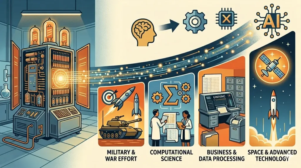
During World War II, first generation computers and their immediate predecessors proved that electronic machines could contribute directly to military outcomes. ENIAC accelerated ballistics calculations that improved artillery accuracy. Codebreaking machines at Bletchley Park, while not strictly first generation in the sense used here, helped break German and Japanese codes and shortened the war. This wartime demonstration of computing power secured enormous post-war government and military investment in computing research.
In the post-war scientific environment, first generation computers enabled the computational science that made nuclear technology, jet propulsion, advanced materials research, and ultimately the space programme possible. Complex simulations that would have taken human teams decades could be completed in days or weeks. Fields like meteorology, which depend on processing enormous quantities of numerical data, were transformed by the availability of electronic computers.
From a business perspective, UNIVAC I, IBM 650, and LEO I demonstrated that computers could automate commercial data processing tasks at a scale and speed that transformed the economics of information management. This opened the door to the computing industry as we know it today, the vast global enterprise of hardware manufacturing, software development, and digital services.
Most fundamentally, first generation computers proved the concept. They showed that machines built from electronic components could perform logical and mathematical operations, that these machines could be programmed to solve a wide range of problems, and that the benefits of this capability justified enormous investments. Every subsequent generation of computer development, right through to the smartphones, cloud servers, and artificial intelligence systems of today, flows from the foundations laid by these first machines.
First Generation Computers vs Second Generation Computers
Understanding how first generation computers compare to their successors helps clarify both the achievements of the first generation and the reasons for the rapid technological transition that followed. The second generation, from approximately 1956 to 1963, replaced vacuum tubes with transistors, which were smaller, cheaper, more reliable, and consumed far less power.
| Feature | First Generation (1940-1956) | Second Generation (1956-1963) |
| Core Technology | Vacuum Tubes | Transistors |
| Physical Size | Very large, often room-filling | Considerably smaller |
| Power Consumption | Extremely high (e.g. 150 kW for ENIAC) | Much lower |
| Reliability | Low, frequent tube failures | Higher, transistors more durable |
| Heat Generation | Very high, required industrial cooling | Moderate, simpler cooling |
| Programming Language | Machine language (binary) | Assembly language |
| Cost | Extremely high | Lower but still expensive |
| Speed | Thousands of operations per second | Hundreds of thousands per second |
| Memory Technology | Magnetic drum, delay lines, CRT tubes | Magnetic core memory |
| Commercial Availability | Very limited | Broader commercial availability |
The transition from first to second generation was driven primarily by the invention of the transistor at Bell Laboratories in 1947. By the mid-1950s, transistors had been developed to a point where they could be manufactured reliably and incorporated into computer designs.
The improvements were dramatic across every dimension: transistors were roughly 100 times smaller than vacuum tubes, consumed far less power, generated far less heat, lasted essentially indefinitely compared to the limited lifespan of vacuum tubes, and could switch on and off far faster.
The IBM 7090, a second-generation machine introduced in 1959, was about 100 times faster than the IBM 704, a contemporary first-generation machine, and far more reliable.
FAQs About Examples of First Generation Computers
1. What are the examples of first generation computers?
The main examples of first generation computers include ENIAC (1945), UNIVAC I (1951), IBM 701 (1952), IBM 650 (1953), EDVAC (1949), EDSAC (1949), LEO I (1951), MANIAC (1952), the IAS Computer (1952), and Harvard Mark I (1944). Each of these machines made a unique contribution to computing history and together they define the first generation era from approximately 1940 to 1956.
2. Which was the first generation computer ever made?
The Harvard Mark I (1944) was one of the earliest large-scale automatic computing machines, though it was electromechanical rather than purely electronic.
ENIAC, completed in 1945, is generally considered the first fully electronic general-purpose digital computer and is the most commonly cited starting point of the first generation of computers. Some historians also point to earlier electronic computing experiments and the British Colossus machine (1943) as precursors, but ENIAC is the most widely recognised first example.
3. What technology did first generation computers use?
First generation computers used vacuum tubes as their primary electronic switching components. Vacuum tubes are sealed glass cylinders that control electrical current flow and act as binary on/off switches. In addition to vacuum tubes, these machines used various memory technologies including mercury delay lines, magnetic drum memory, and Williams tube electrostatic storage. Data was typically input through punch cards or paper tape and output through printers or punch card machines.
4. How many first generation computers were built?
The total number depends on how the category is defined. Genuinely one-of-a-kind research machines like ENIAC, EDVAC, EDSAC, IAS, and MANIAC were each built as single units. The IBM 701 was produced in nineteen units. The UNIVAC I saw 46 systems delivered.
The IBM 650 was the most widely produced first generation computer with over 2,000 units manufactured, making it the first computer produced in genuinely commercial quantities. Across all models, the total number of first generation computers ever built is in the low thousands.
5. What is the difference between first and second generation computers?
The fundamental difference is the core switching technology. First generation computers used vacuum tubes, which were large, power-hungry, heat-producing, and fragile. Second generation computers replaced vacuum tubes with transistors, which were much smaller, consumed far less power, produced far less heat, and were vastly more reliable.
This technological change produced computers that were significantly smaller, cheaper, faster, and more practical than their first generation predecessors. Second generation computers also introduced assembly language programming, replacing the pure binary machine language of the first generation.
6. Which first generation computer was used for business?
Several first generation computers were used for business purposes. LEO I, built by J. Lyons and Company in the United Kingdom and operational from 1951, was the first computer specifically designed and used for commercial business data processing, handling payroll, inventory, and financial calculations.
UNIVAC I, from 1951, was the first commercially sold computer in the United States and was widely adopted by businesses and government agencies for data processing tasks. The IBM 650, introduced in 1953, became the most widely sold first generation computer and was extensively used by businesses, universities, and government organisations.
7. Is Harvard Mark I a first generation computer?
The Harvard Mark I occupies a somewhat transitional position. It is generally included in discussions of first generation computers because of its era (completed in 1944) and its significance as an early large-scale automatic computing machine.
However, it is technically an electromechanical computer using relay switches and mechanical components rather than a purely electronic machine using vacuum tubes. Some historians classify it as a pre-first-generation or zero-generation computer. For most practical purposes and in most educational contexts, it is included in the first generation category due to its historical importance and the era in which it operated.
Conclusion
The examples of first generation computers we have explored in this guide, from the room-filling ENIAC to the business-oriented LEO I, from the architecturally revolutionary EDVAC to the academically influential EDSAC, collectively represent one of the most remarkable engineering achievements in human history. These machines were built with technologies and methods that seem almost impossibly primitive by modern standards, yet they accomplished things that had never been done before and opened intellectual doors that could never be closed again.
Each machine contributed something unique. ENIAC proved electronic computing was possible and practical. UNIVAC I demonstrated it could be commercially viable. IBM 701 and 650 built the computing industry. EDVAC and IAS established the architectural principles that still govern computer design today.
EDSAC proved computers could serve science. LEO I proved they could transform business. MANIAC and IAS pushed the boundaries of scientific computation. Harvard Mark I bridged the mechanical and electronic eras. Together, they built the foundation of the digital world.
Understanding these first generation computers matters not just as historical curiosity but as context for appreciating how profoundly technology shapes human capability and possibility.
The trajectory from ENIAC in 1945 to the artificial intelligence systems of today took less than eighty years, a span of time shorter than a single human lifetime. That trajectory began with these first machines, humming and clicking in specially built rooms, attended by teams of engineers, solving problems that would change the world.
To deepen your understanding of computing history and hardware fundamentals, explore our related guides on What Is First Generation Computer, Generations of Computers, What Is Computer Hardware, and Second Generation Computers. Each guide builds on the foundations laid in this article and brings you closer to a complete understanding of how modern computer systems came to be.